Understanding Convolutional Neural Network (CNN) — A Guide to Visual Recognition in the AI Era

Author(s): Sanket Rajaram

Originally published on Towards AI.

Understanding Convolutional Neural Network (CNN) — A Guide to Visual Recognition in the AI Era

This article will help you understand the application of conventional artificial neural networks to visual recognition problems. We’ll understand the basics of convolutional neural networks with different image processing strategies for feature generation with dimensionality reduction techniques for improving computational complexity.

The goal of this article is to provide a deeper understanding of structural design changes made into a traditional artificial neural network to solve real-world problems in the field of image processing.

We’ll start from basics of design components such as convolution over single-channel and multi-channel images with different sized kernels for feature map generation and move on to pooling operation for subsampling. Further, we will cover the building blocks of convolutional neural networks like convolution layer, pooling layer and hyperparameters such as convolution strides, padding.

With this article, you will able to understand how to practically implement a convolutional neural architecture with different components as convolution, pooling, and fully-connected neural network architecture in TensorFlow 2.0.

This article discusses the classical convolutional neural network architecture, LeNet-5 which consists of a stacked architecture of convolutional layers for feature map generation and pooling layers for feature subsampling followed by a multi-layered fully-connected feed-forward neural network for multi-label classification.

You will also get an insight on how to design an artificial neural network for the most common use cases as image classification, object detection without any use of rule-based hand-crafted feature detection algorithms and with the more generalized form of the visual recognition architecture.

In this article, we’re going to cover the following main topics:

• Introduction to Conventional Visual Recognition
• Building Blocks of Convolutional Neural Network (CNN)
• Designing a Convolutional Neural Network Architecture
• LeNet-5 — A Classical Neural Network Architecture
• Implementing Convolutional Neural Network with TensorFlow 2.0

Technical requirements

The program code is written and run in a Google Colab Notebook Service offered by Google Inc. The installation instructions are given in respective sections as per the requirements.

Introduction to Conventional Visual Recognition

In this section, we will take the brief overview of digital image processing including how an image is processed algorithmically, what will happen if we feed the matrix of pixels to an artificial neural network, how we can reduce the spatial dimension of image data, how the conventional neural network architectures like multi-layered perceptron perform with image transformations. This section elaborates the inefficiencies of using the traditional hand-crafted rule-based feature detection algorithms which are unable to exhibit invariance to image translations and computationally expensive architectures.

What is Digital Image Processing

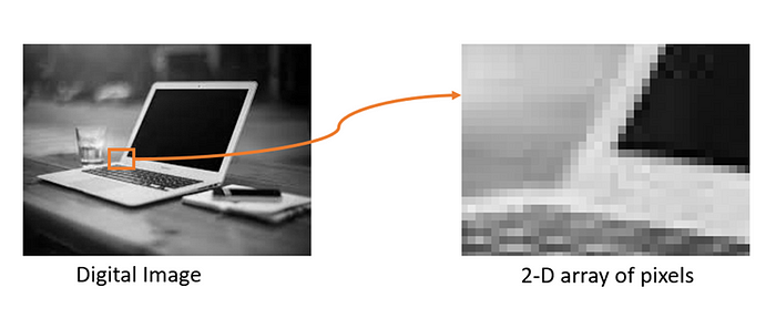
Digital image processing is a way of applying a set of sophisticated techniques and algorithms to digital images to enhance, optimize, and extract useful information. The structure of the image is mainly composed of a dimensional array of picture elements called pixels.

An image is rendered as a dimensional matrix of pixels as shown in the following figure where the number of rows represents the height of the image and the number of columns represents the width of the image.

Dimensions of a digital image are the height and width of the image measured in terms of the pixel. A picture element (pixel) represents the brightness or colour intensity value. In the case of a grayscale image, it ranges from 0 to 255, shades of black and white. While in the colour image, it ranges from 0 to 255 for the individual red, green, and blue channels.

Computer vision is one of the key areas in artificial intelligence that tries to mimic the human visual system in a way to perceive and enable computing devices to understand and process information in images and videos. Until now, this field possessed limited capabilities for extracting and processing features in images and videos but now the deep neural networks are helping computers to surpass human ability in some tasks of detecting and tagging objects in images.

One of the key factors in the rapid development of efficient prototypes in computer vision is the advancement in the smartphone technologies with which we have more images and videos to train artificial neural networks more efficiently and improve the ability of computers to visualize objects in an image.

In the traditional rule-based algorithmic systems, objects in the image are typically identified with the help of feature detection algorithms. For example, to detect the edges of an object in an image, we use edge detection algorithms like Sobel and Prewitt, whereas to detect corners of an object, we use corner detection techniques like Harris.

For more robust feature detection, invariant features like scale-invariant feature transform (SIFT) and speed-up robust features (SURF) are used, but these features are designed to work in a limited context and fail to generalize. Their context is limited to object identification tasks while neural networks have outperformed in image classification and retrieval tasks.

Artificial Neural Network for Digital Image Processing

One of the key problems in computer vision is the size of input data as it can be big. Assume we have a color image of size 16 by 16 pixels, as shown in the following figure. As it is a color image, it has red, green, and blue channels; thus, the total number of pixels in this image is 16 x 16 x 3, which is 768 pixels. Assuming this is the input data size for a neural network which is still a manageable size for a neural network to process.

In a multi-layered neural network, if the input data size is 768, then possibly a network will have several thousands of parameters or weights to process. But in case of large-sized images, say a color image with 1200 by 800 pixels resolution will have 28,80,000 pixels which will be a huge sized input as it will have millions of parameters to process for a neural network, which is highly time-consuming and an inefficient way of dealing with imagery form of data.

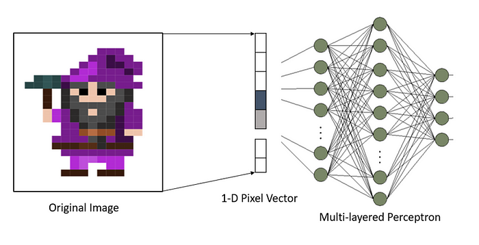
To train a neural network with a billion parameters is computationally expensive and can lead to overfitting of the learning model due to difficulty in exploring different weight values for the neural networks. Thus, a multi-layered perceptron is not a good choice for high-dimensional data like images.

Another problem with a multi-layered perceptron is that it does not perform well with image transformations. If we feed an image by flattening its matrix of pixels into a vector form and feed it to a fully-layered neural network, then a neural network reacts differently to different transformations of the same input image.

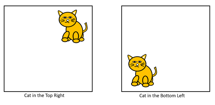
If a cat appears in the top right corner of one image and in the bottom left corner of another image, as shown in the following figure, then the ordinary neural network will learn these images as different images though they have the same cat object. So, the multi-layered neural network is not suitable for tasks like object detection and image classification due to its inability to retain invariance against different transformations of the same image.

The multi-layered perceptron has one more drawback. When a matrix of pixels is transformed into a vector by rendering the pixel values row-by-row, as shown in the following figure, then spatial information is lost as there exists a spatial correlation between neighboring pixels than consecutive pixels.

Thus, we require a possible solution to retain the spatial correlation of the features in an image and which is invariant to position and scale changes. A better solution can be a convolutional neural network (CNN), a form of artificial neural network designed for analyzing imagery data. CNN is a highly efficient form of neural network which is invariant to spatial transformations.

Building Blocks of Convolutional Neural Network

Let us first understand the various components of the convolutional neural network. In this section, we will study convolution, padding, strides, and pooling in the context of image processing. As well we will study various hyperparameters like convolution strides, padding, zero padding, and border pixel padding, which affect the computational complexity of convolutional neural network architecture.

Convolution over 2D Image

A convolution operation is one of the important stages of a convolutional neural network. In the process of convolution, a kernel window slides over an image row-wise from left to right doing elementwise multiplication and aggregate the result with summation. The output of convolution operation varies with respect to values in the kernel.

Convolution operation typically performs an element-wise multiplication of the window of pixels with the kernel matrix and then aggregates with summation as shown in the following figure. In this example, we have used a filter of size 3 x 3 which can detect edges from the 2D image. It typically performs iterative multiplication with a sliding window of pixels and sum all these multiplication values at the end.

In the case of 3D images like color images, the shape of images changes. In the above example, a gray-scale image is considered for convolution where it has only two dimensions, that are height and width, while in the case of color images, there are three dimensions that are height, width, and depth of the image, where depth corresponds to a number of color channels. So, to detect basic features like edges or corners in an image, the convolution operation performs the convolution of a matrix of pixels with different kernels. This is done to generate a unique set of feature maps that represent the spatial correlation among the neighboring pixels.

Convolution over 3D Image

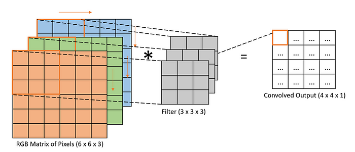
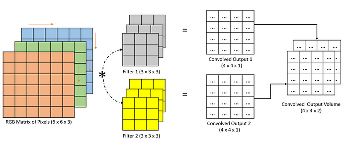
3D images typically have three dimensions: height, width, and depth. Consider an image of shape 6×6×3 that represents height as 6, width as 6, and depth as 3 that corresponds to the three color channels in the image. We can think of this as a stack of three 6×6 images. In order to detect edges or some other feature in the 3D image, we convolve it with a 3 x 3 × 3 stacked layers of filter.

Convolution with Multiple Filters

If we are going to use multiple filters and convolve them with the input matrix of pixels, it will generate multiple outputs representing the volume of outputs as shown in the following figure. In this example, an RGB image of shape 6 x 6 x 3 is convolved with two different filters having a size of 3 x 3 x3 generating the stack of convolved outputs with a size of 4 x 4 x 2. In the convolutional neural network, a similar kind of strategy is used to get multiple representative feature maps of the image.

Padding

With the convolution operation, the size of the image gets shrunk to the extent of the size of the kernel and the number of strides. If you take a gray-scale image, a matrix of gray pixel values, and perform convolution on it with some kernel, it should be noted that in the process of convolution the centrally-located pixels are covered more than once than the boundary pixels. So, this process of convolution has two drawbacks, shrinking image as output of convolution and loss of Information as boundary pixels are not well-represented in the convolution process.

To surmount these drawbacks, we can use a padding mechanism, where we will add an extra layer of values, either with zero or boundary values. In the following figure, the original matrix of pixels is padded with one extra layer of values. There are two options for padding, zero-padding by adding an extra layer of zeros surrounding border pixels and border pixel padding by adding an extra layer with the repetition of border pixels. In the following figure, an original matrix is padded with a layer of zeros and border pixels, here the size of padding =1.

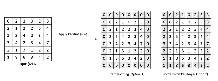
We can add multiple layers of padding as per the requirements to retain the original dimension of the image. In the following figure, the addition of an extra layer around the border pixels has changed the original dimension of an image, but it will help in retaining the size of the image after the convolution process.

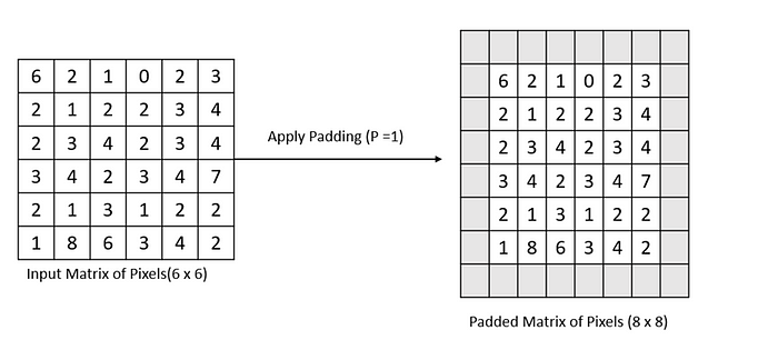
As seen in the following figure of convolution, an image of size, 6 x 6 convolves with a filter of 3 x 3, it returns a convolved image with a size of 4 x 4 as no padding is used in convolution process. This is known as valid convolution.

But in the following figure, a matrix of pixels is first zero-padded and then convolved with edge filter, this results in preservation of the original dimension of an image, this convolution is called as the same convolution. In the following figure, the size of the output is equal to the size of the input.

The padding mechanism helps in the retention of the original dimensions of an image and also helps in preventing the loss of information in the border pixels. In general, if we assume the input dimension of the image is Iₕ x Iᵥ that represents the height and width of the image, respectively and the kernel with dimension Kₕ x Kᵥ that represents the height and width of the kernel window, then the dimension of convolved image is height, (Iₕ x Kₕ + 1) and with width, (Iᵥ x Kᵥ + 1). Hence it clearly shows that the dimensions of output are dependent on the shape of input and the shape of the kernel window.

If we convolve an image with a shape, 500 x 500 pixels and convolve it with 10 layers of 5 x 5 kernel, it will reduce the shape of the image to 460 x 460 because a single convolution with 5 x 5 kernel will reduce the shape of input by 4, resulting into reduction of near to 10% of the image. So, this issue of shrinking an image over multiple convolutions can be resolved by the padding mechanism.

If p represents the padding size for input image then after convolution the dimensions of output, height as (Iₕ-Kₕ+2p+1) and width as (Iᵥ-Kᵥ+2p+1)). This shows that the dimensions of output will increase by p.

Convolutional operations typically use odd-sized kernel window such as 3, 5 or 7. Selecting the odd-sized kernel helps in retaining spatial dimensionality and as well helps in applying the same padding around the border pixels.

Convolution Strides

Strides decide by how many blocks of pixel a kernel window should move row-by-row from left-to-right. Strides play an important role in the assessment of information gain with convolution operation over different-sized window movements. As shown in the following figure, a matrix of pixels convolves with a kernel of size 3 x 3 in left-to-right direction with a number of strides at first, S = 1, which is the most usual practice in convolution operation. While with Strides, S = 2, a kernel window moves by two blocks of pixel resulting in much shrinkage of the dimension of the original image.

Strided convolutions are highly popular for reducing the higher dimensions of an image drastically. For retaining computational efficiency, we can down sample the input matrix of pixels with strides. Assuming the convolution padding size as p, the kernel size as k, convolution strides as S, and the height and width of output feature maps (Oₕ, Oᵥ) the dimensions of output will change to,

In summary, padding can help in preserving the dimensions of an image after convolution operation and helps to cover border pixels to regain information. While a convolution stride helps in down sampling of the dimensions of the input image, in turn, resulting in reducing the dimensions of the output image.

Pooling Operation

Pooling operation is an important building block of a convolutional neural network. Pooling helps in dimensionality reduction without losing information. It helps in reducing spatial dimensions of the feature maps which in turn helps in reducing the trainable parameters and effectively reducing the computational complexity of the neural network.

The most commonly used pooling approaches are average pooling and max pooling. The pooling operation involves the screening of each channel of the feature map by sliding a 2-dimensional window over it and summarizing the features in that window with the maximum or average value. Consider a feature map of shape Iₕ x Iᵥ x Iₐ, the pooling operation changes the dimension of this feature map to,

In this equation, Iₕ represents the height of the feature map, Iᵥ represents the width of feature map and Iₐ represents the number of channels in the feature map with k x k sized filter and number of strides as S.

In the max pooling operation, a maximum value is selected over a screening region or a feature map; this region represents the size of the filter. After the max-pooling operation, the feature map is subsampled to the most representative set of features, as shown in the following figure, where a feature map of shape 6 x 6 is filtered by window size 2 x 2 and a number of strides as 2, resulting in the set of maximum values preserving the most relevant features of the feature map.

While, in case of average pooling operation, an average feature value is calculated over the filter window as shown in the following figure. Here, an input feature map of size 6 x 6 is filtered over a sliding window size of 2 x 2 with a number of strides as 2 resulting into the set of average feature values representing the group of features in the regional window.

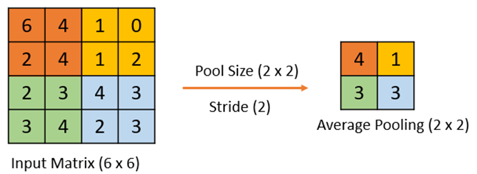
In most convolutional neural networks, the convolutional layers and pooling layers are stacked consecutively to retain prominent feature maps with a reduction in spatial complexity. The pooling layer is typically used to reduce the dimensions of the feature map that is generated with convolution operation resulting in a smaller number of trainable parameters and summarization of feature maps effectively without loss of information.

Designing a Convolutional Neural Network Architecture

In this section, we will design our first convolutional neural network architecture with the different components that we studied in the previous section. We will build a stacked architecture of layers that are sequentially arranged to generate a unique set of features from multiple consecutive layers of convolution and pooling operation, then finally feed into a fully connected layer of neurons for learning non-linear relationships within the feature maps with a gradient descent optimization algorithm.

Design of First Layer of CNN Architecture

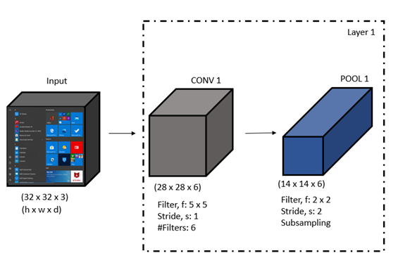
In the very first layer of a CNN architecture, an input multi-channel color image of shape 32 x 32 x 3 representing height, width, and number of channels in an image, respectively, is convolved with a kernel of size 5 x 5; the number of kernels is 6 with a number of strides as 1. This convolution operation will generate a feature map of size 28 x 28 x 6. This bunch of feature maps is subsampled with a max pooling operation with pool size as 2 x 2 and a number of strides as 2, resulting in a down-sampled feature map of shape 14 x 14 x 6 as shown in the following figure. Here, we have assumed that a layer is a collective representation of the convolution and pooling layer.

Design of Second Layer of CNN Architecture

In the second layer of CNN architecture, another set of convolution and pooling operations is added, as shown in the following figure. This layer of CNN firstly performs a convolution of input feature maps generated in the first layer with a kernel of size 5 x 5 with a greater number of filters to further create a more minimalistic representation of an original image in the form of feature maps. Further, in this layer of CNN architecture, a feature map generated from a convolution operation is subsampled with a pooling operation to reduce the spatial dimensions of feature maps.

Design of Flattened Fully Connected Layer of CNN Architecture

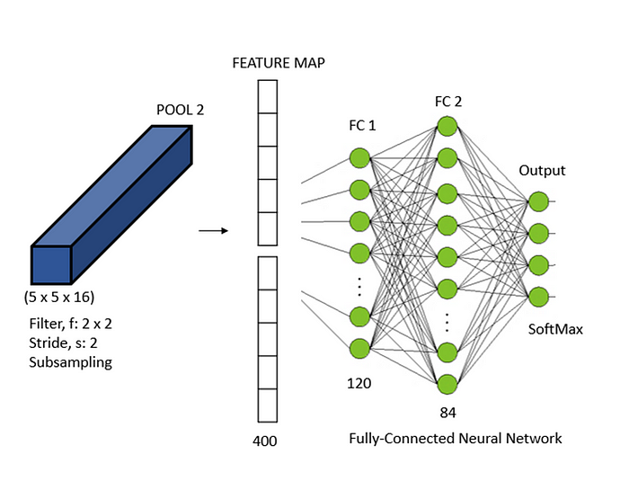
In the third layer of CNN architecture, the feature maps generated with previous layers are flattened into a vector form and fed into a fully connected layer of size 120 and subsequently to another fully connected neural layer of size 84, finally fed to an output layer of multi-label SoftMax classifier.

The SoftMax Activation function helps to normalize the output of the neural network and transforms it into a probability distribution over predicted output classes.

The important characteristic of Convolutional Neural Networks (CNN) is that a learning model is highly translation-invariant. It means a CNN model trained with a pattern in the top-right corner of the image can detect similar patterns in any corner of the image regardless of its location in the image. This would not have been possible merely with the conventional neural networks without the use of multiple sets of convolution and pooling layers. This makes the CNN a more generalized form of neural network for visual recognition systems.

A learning model built from CNN is able to learn spatial relationships of patterns with its ability to learn more complex relationships in visual concepts. In the first layer of convolution, a learning model learns the basic features in an image, like edges, and corners, while in the subsequent layers of convolution, it learns the complex features in the image, like objects in the image.

So, in this section, we have studied the different layers of convolutional neural networks with their abilities to learn the inherent nature of the data.

In the next section, we will learn a benchmark neural network architecture, LeNet-5 and its design components.

LeNet-5 — A Classical Neural Network Architecture

The LeNet-5 architecture is a benchmark example of a convolutional neural network which was used to automatically classify the handwritten digits. The LeNe5–5 has mainly the sets of convolutional and pooling layers followed by a flattened fully-connected layer of neural network with a SoftMax classifier for classifying the digit image into different classes ranging from 0 to 9.

LeNet is one of the important neural architecture which made the rule-based feature extraction algorithms redundant with ability to automatically learn the inherent features of a raw image.

The LeNet-5 has mainly three different types of layers, convolutional layers (CONV1, CONV2, CONV3), subsampling layers (POOL1, POOL2), and a fully-connected neural layer (FC1), followed by the output layers shown in the following figure.

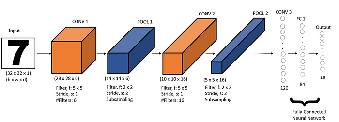
The CONV1 layer takes an input matrix of pixels of shape, 32 x 32 x 1 representing height, width, and depth of input, respectively. CONV1 convolves an input matrix of 32 x 32 x 1 with 6 kernels each of shape 5 x 5 with stride as 1, this generates a convolved output of size 28 x 28 x 6. This data is passed for the next phase of the pooling layer, POOL1, where an average pooling operation is performed with a filter of size of 2 x 2 and stride as 2, resulting in a sub-sampled output of size 14 x 14 x 6.

In the next stage, CONV2, convolution is performed with 16 filters of size 5 x 5 and stride as 1 that gives a convolved output of 10 x 10 x 16. This is convolved output is sub-sampled with another average pooling layer, POOL2 in which the size of data further reduced in dimensions as 5 x 5 x 16. This sub-sampled output is flattened into a vector of 400 x 1 and passed to the next layer in the LeNet-5, which is a fully-connected convolutional layer, CONV3, which takes the values from the input vector.

Each of the nodes in this layer of size 120 is connected to every feature value in that vector. The next layer in the LeNet-5 is a fully-connected neural layer having 84 nodes. This is finally connected to an output layer having 10 probable values ranging from 0 to 9. In the LeNet-5 architecture the sigmoid/tanh activation functions have been used.

Summary of LeNet-5 architecture is shown in the following figure,

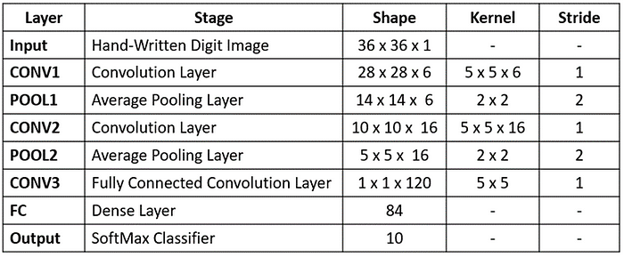
The LeNet-5 architecture was able to attain an error rate below 1% on the popular MNIST dataset consisting of images handwritten digits. Thus, in this section, we tried to understand the classical convolutional neural network architecture with its building blocks such as convolution layer, pooling layer and fully-connected neural network layer for hand-written digit classification without use of hand-crafted feature detection algorithms.

Implementing Convolutional Neural Network with TensorFlow 2.0

In this section, we will build a well-structured convolutional neural network architecture with TensorFlow 2.0.

With the help of Keras library, now part of TensorFlow 2.0, it has become lot easier to design complex neural network architectures with ability of debugging the program efficiently.

1. Let us at first import the required libraries in the program environment as follows,

from tensorflow import keras

2. After importing the Keras library from TensorFlow 2.0, we will define a sequential model which allows to build a group of linear stack of layers as follows with the Sequential() method from Keras library.

model_structure=keras.models.Sequential()

3. Let us now add a first convolutional layer with a kernel size of 5 x 5, a number of filters as 10 with the same padding, and RELU as an activation function with add() method. This layer of convolution will take an input image of a shape 28 x 28 x 1. After the convolutional layer, a feature map gets generated, which we will subsample with the max pooling layer of size 2 x 2 with the add() method, which will add a layer instance on the top of the convolutional layer.

model_structure.add(keras.layers.Conv2D(10, (5, 5),padding='same', activation='relu', input_shape=(28, 28, 1)))
model_structure.add(keras.layers.MaxPooling2D((2, 2)))

4. Let us add one more group of convolution and pooling layers in the layered stack with a greater number of filters as 16 as follows,

model_structure.add(keras.layers.Conv2D(16, (5, 5),padding='same' ,activation='relu'))
model_structure.add(keras.layers.MaxPooling2D((2, 2)))

5. Furthermore, add another layer of group of the convolutional layer with a kernel size of 3 x 3 and number of filters as 64 and max pooling layer as follows,

model_structure.add(keras.layers.Conv2D(64, (3, 3),padding='same', activation='relu'))
model_structure.add(keras.layers.MaxPooling2D((2, 2)))

6. Let us now flatten the layers of feature maps generated by multiple groups of convolution and pooling to feed into a fully-connected neural network of shape 120 and activation function as RELU. More non-linearity is introduced by adding another fully-connected layer as size 80 and finally a SoftMax layer is added for multi-label classification of images as follows,

model_structure.add(keras.layers.Flatten())
model_structure.add(keras.layers.Dense(120, activation='relu'))
model_structure.add(keras.layers.Dense(80, activation='relu'))
model_structure.add(keras.layers.Dense(10, activation='softmax'))

7. A summary of sequential model can be obtained by using summary() method.

model_structure.summary()

Output of above line of code is as follows which clearly shows the layer-wise trainable parameters to be learned by neural network architecture.

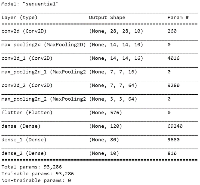
Let us now understand the calculation of trainable parameters,

• The first input layer has no trainable parameters.
• The first CONV2D layer uses a kernel size 5 x 5 and number of filters as 10, so the trainable parameters are equal to (shape of kernel x number of filters) + bias value of each filter that result becomes, ((5 x 5) x 10) + 10 is equal to 260 trainable parameters.
• The first Maxpoling2D layer has no parameters.
• The second CONV2D layer uses a kernel size 5 x 5 and number of filters as 16, so the trainable parameters are equal to ((shape of kernel x number of filters) x number of filters in the previous convolution layer + bias value of each filter that result becomes, ((5 x 5) x 16 ) x 10 + 16 is equal to 4016 trainable parameters.
• The second Maxpoling2D layer has no parameters.
• The third CONV2D layer uses a kernel size 3 x 3 and number of filters as 64, so the trainable parameters are equal to ((shape of kernel x number of filters) x number of filters in the previous convolution layer + bias value of each filter that result becomes, ((3 x 3) x 64) x 16 + 16 is equal to 9280 trainable parameters.
• The third Maxpoling2D layer has no parameters to train.
• The first fully-connected layer, Dense takes input feature vector of size 576 and has 120 nodes which in turn has (input shape x number of nodes) connections + bias for each node that is equal to (576 x 120) + 120 becomes 69240 trainable parameters.
• The second fully-connected layer, Dense_1 takes input feature vector of size 120 and has 80 nodes which in turn has (input shape x number of nodes) connections + bias for each node that is equal to (120 x 80) + 80 becomes 9680 trainable parameters.
• The third fully-connected layer, Dense_2 takes input feature vector of size 80 and has 10 nodes which in turn has (input shape x number of nodes) connections + bias for each node that is equal to (80 x 10) + 10 becomes 810 trainable parameters.

Thus, we have practically implemented a convolutional neural network with set of convolutional layers, pooling layers and fully-connected dense neural network layers with configuration of various hyperparameters as number of filters, kernel size, number of strides, pool size and activation functions.

Summary

In this article, we learned the different challenges that we face in solving computer vision problems, starting with the basics of digital image processing, applying conventional neural networks for image recognition problems, and its shortcomings like more expensive computational complexity for high-dimensional data like images and susceptibility to geometric transformations.

We learned different building blocks of the convolutional neural network. We started with how convolution operation generates the feature map with different types of kernels on single and multi-channel images. Then, we studied stride convolution used for dimensionality reduction with different sized strides along with padding variants like zero padding which helps to regain the original dimension of the image.

We studied the pooling operation, a technique used for delimiting the most prominent portions of an image. Pooling helps in advancing computational efficiency of learning feature maps of the image. After studying different components of convolutional neural network architecture, we designed a simple stacked-layer of convolution and pooling layers, followed by fully-connected neural network layers and finally fed to multi-label classification layer for image recognition problem.

We studied the classical convolutional network architecture, LeNet-5 along with its different layers. Finally, we built a simple convolutional neural network architecture with TensorFlow 2.0.

Join thousands of data leaders on the AI newsletter. Join over 80,000 subscribers and keep up to date with the latest developments in AI. From research to projects and ideas. If you are building an AI startup, an AI-related product, or a service, we invite you to consider becoming a sponsor.

Published via Towards AI