Main Types of Neural Networks and its Applications — Tutorial

Nowadays, there are many types of neural networks in deep learning which are used for different purposes. In this article, we will go through the most used topologies in neural networks, briefly introduce how they work, along some of their applications to real-world challenges.

📚 This article is our third tutorial on neural networks, to start with our first one, check out neural networks from scratch with Python code and math in detail. 📚

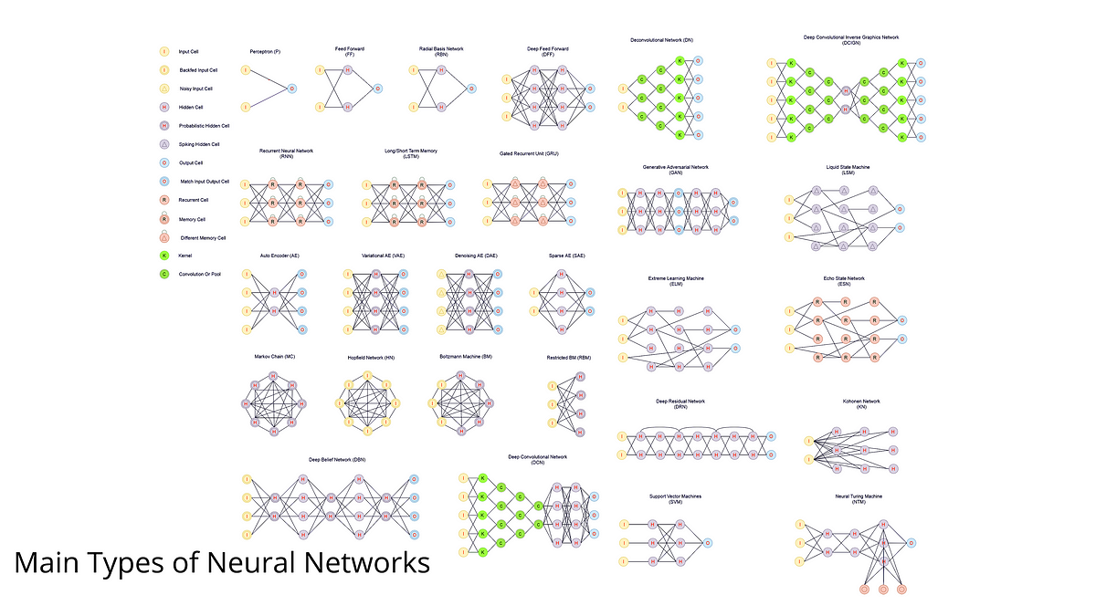
Neural Network Topologies

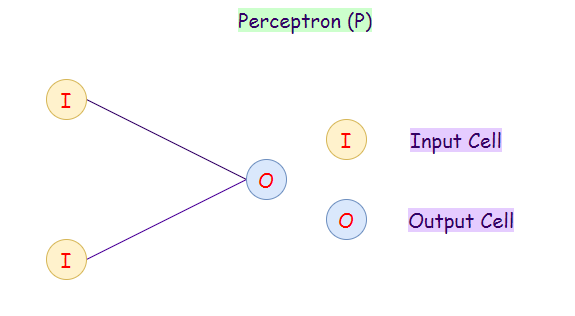
1. Perceptron (P):

The perceptron model is also known as a single-layer neural network. This neural net contains only two layers:

• Input Layer
• Output Layer

In this type of neural network, there are no hidden layers. It takes an input and calculates the weighted input for each node. Afterward, it uses an activation function (mostly a sigmoid function) for classification purposes.

Applications:

• Classification.
• Encode Database (Multilayer Perceptron).
• Monitor Access Data (Multilayer Perceptron).

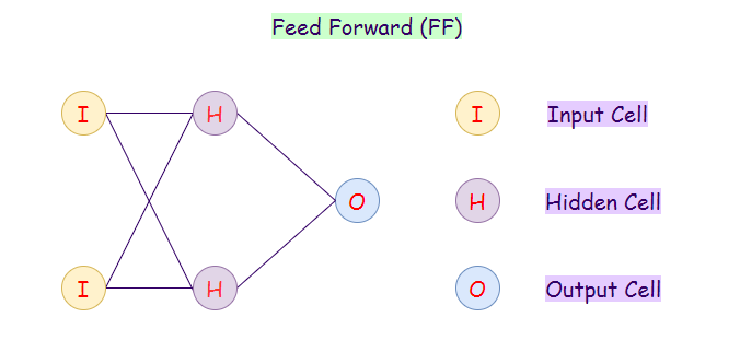
2. Feed Forward (FF):

A feed-forward neural network is an artificial neural network in which the nodes do not ever form a cycle. In this neural network, all of the perceptrons are arranged in layers where the input layer takes in input, and the output layer generates output. The hidden layers have no connection with the outer world; that’s why they are called hidden layers. In a feed-forward neural network, every perceptron in one layer is connected with each node in the next layer. Therefore, all the nodes are fully connected. Something else to notice is that there is no visible or invisible connection between the nodes in the same layer. There are no back-loops in the feed-forward network. Hence, to minimize the error in prediction, we generally use the backpropagation algorithm to update the weight values.

Applications:

• Data Compression.
• Pattern Recognition.
• Computer Vision.
• Sonar Target Recognition.
• Speech Recognition.
• Handwritten Characters Recognition.

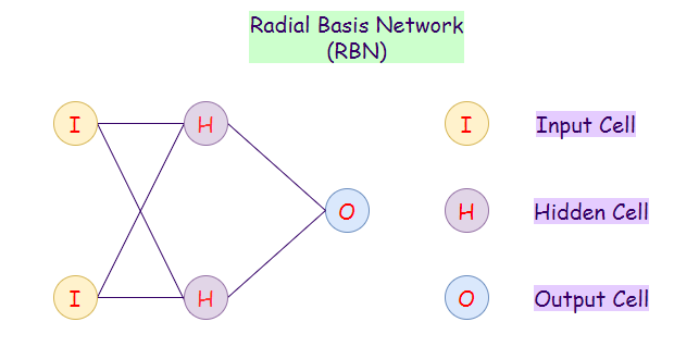
3. Radial Basis Network (RBN):

Radial basis function networks are generally used for function approximation problems. They can be distinguished from other neural networks because of their faster learning rate and universal approximation. The main difference between Radial Basis Networks and Feed-forward networks is that RBNs use a Radial Basis Function as an activation function. A logistic function (sigmoid function) gives an output between 0 and 1, to find whether the answer is yes or no. The problem with this is that if we have continuous values, then an RBN can’t be used. RBIs determines how far is our generated output from the target output. These can be very useful in case of continuous values. In summary, RBIs behave as FF networks using different activation functions.

Applications:

• Function Approximation.
• Timeseries Prediction.
• Classification.
• System Control.

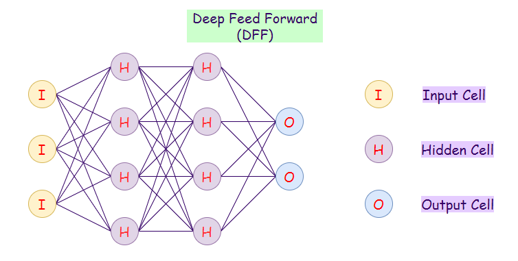
4. Deep Feed-forward (DFF):

A deep feed-forward network is a feed-forward network that uses more than one hidden layer. The main problem with using only one hidden layer is the one of overfitting, therefore by adding more hidden layers, we may achieve (not in all cases) reduced overfitting and improved generalization.

Applications:

• Data Compression.
• Pattern Recognition.
• Computer Vision.
• ECG Noise Filtering.
• Financial Prediction.

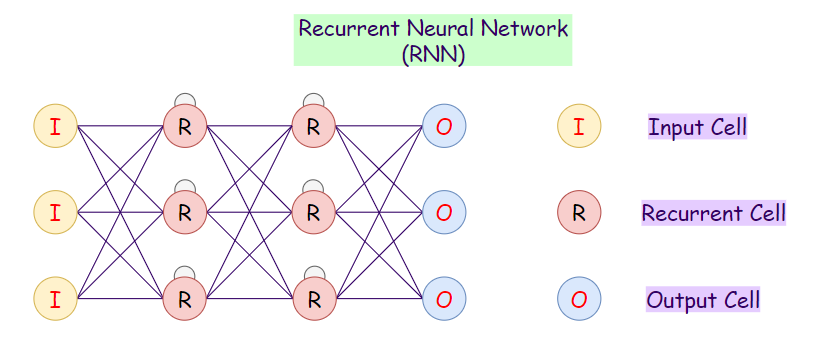
5. Recurrent Neural Network (RNN):

Recurrent neural networks (RNNs) are a variation to feed-forward (FF) networks. In this type, each of the neurons in hidden layers receives an input with a specific delay in time. We use this type of neural network where we need to access previous information in current iterations. For example, when we are trying to predict the next word in a sentence, we need to know the previously used words first. RNNs can process inputs and share any lengths and weights across time. The model size does not increase with the size of the input, and the computations in this model take into account the historical information. However, the problem with this neural network is the slow computational speed. Moreover, it cannot consider any future input for the current state. It cannot remember info from a long time ago.

Applications:

• Machine Translation.
• Robot Control.
• Time Series Prediction.
• Speech Recognition.
• Speech Synthesis.
• Time Series Anomaly Detection.
• Rhythm Learning.
• Music Composition.

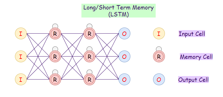
6. Long / Short Term Memory (LSTM):

LSTM networks introduce a memory cell. They can process data with memory gaps. Above, we can notice that we can consider time delay in RNNs, but if our RNN fails when we have a large number of relevant data, and we want to find out relevant data from it, then LSTMs is the way to go. Also, RNNs cannot remember data from a long time ago, in contrast to LSTMs.

Applications:

• Speech Recognition.
• Writing Recognition.

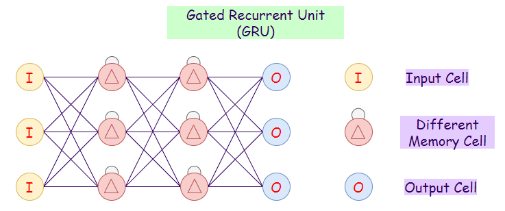
7. Gated Recurrent Unit (GRU):

Gated Recurrent Units are a variation of LSTMs because they both have similar designs and mostly produce equally good results. GRUs only have three gates, and they do not maintain an Internal Cell State.

a. Update Gate: Determines how much past knowledge to pass to the future.
b. Reset Gate: Determines how much past knowledge to forget.
c. Current Memory Gate: Subpart of reset fate.

Applications:

• Polyphonic Music Modeling.
• Speech Signal Modeling.
• Natural Language Processing.

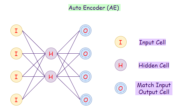
8. Auto Encoder (AE):

An autoencoder neural network is an unsupervised machine learning algorithm. In an autoencoder, the number of hidden cells is smaller than the input cells. The number of input cells in autoencoders equals to the number of output cells. On an AE network, we train it to display the output, which is as close as the fed input, which forces AEs to find common patterns and generalize the data. We use autoencoders for the smaller representation of the input. We can reconstruct the original data from compressed data. The algorithm is relatively simple as AE requires output to be the same as the input.

• Encoder: Convert input data in lower dimensions.
• Decoder: Reconstruct the compressed data.

Applications:

• Classification.
• Clustering.
• Feature Compression.

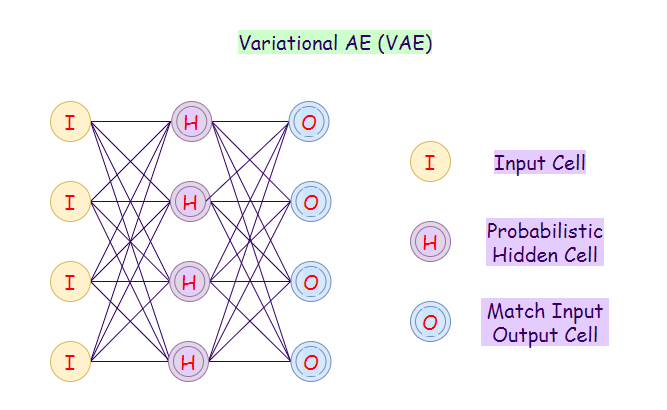
9. Variational Autoencoder (VAE):

A Variational Autoencoder (VAE) uses a probabilistic approach for describing observations. It shows the probability distribution for each attribute in a feature set.

Applications:

• Interpolate Between Sentences.
• Automatic Image Generation.

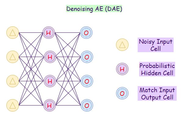
10. Denoising Autoencoder (DAE):

In this autoencoder, the network cannot simply copy the input to its output because the input also contains random noise. On DAEs, we are producing it to reduce the noise and result in meaningful data within it. In this case, the algorithm forces the hidden layer to learn more robust features so that the output is a more refined version of the noisy input.

Applications:

• Feature Extraction.
• Dimensionality Reduction.

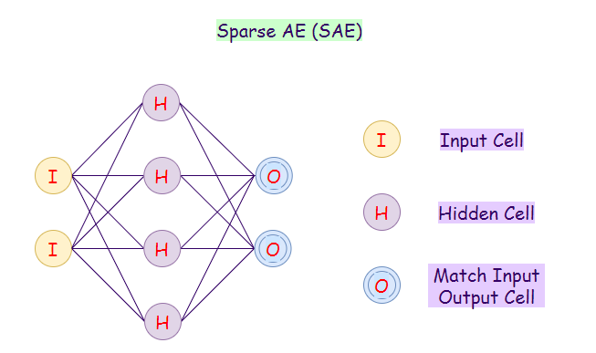
11. Sparse Autoencoder (SAE):

On sparse autoencoder networks, we would construct our loss function by penalizing activations of hidden layers so that only a few nodes are activated when a single sample when we feed it into the network. The intuition behind this method is that, for example, if a person claims to be an expert in subjects A, B, C, and D then the person might be more of a generalist in these subjects. However, if the person only claims to be devoted to subject D, it is likely to anticipate insights from the person’s knowledge of subject D.

Applications:

• Feature Extraction.
• Handwritten digits Recognition.

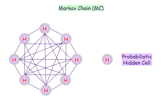
12. Markov Chain (MC):

A Markov chain is a mathematical system that experiences the transition from one state to another based on some probabilistic rules. The probability of transitioning to any particular state is dependent solely on the current state, and time elapsed.

For instance, some set of possible states can be:

• Letters.
• Numbers.
• Weather Conditions.
• Baseball Scores.
• Stock Performances.

Applications:

• Speech Recognition.
• Information And Communication System.
• Queuing Theory.
• Statistics.

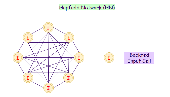
13. Hopfield Network (HN):

In a Hopfield neural network, every neuron is connected with other neurons directly. In this network, a neuron is either ON or OFF. The state of the neurons can change by receiving inputs from other neurons. We generally use Hopfield networks (HNs) to store patterns and memories. When we train a neural network on a set of patterns, it can then recognize the pattern even if it is somewhat distorted or incomplete. It can recognize the complete pattern when we feed it with incomplete input, which returns the best guess.

Applications:

• Optimization Problems.
• Image Detection And Recognition.
• Medical Image Recognition.
• Enhancing X-Ray Images.

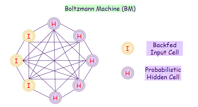
14. Boltzmann Machine (BM):

A Boltzmann machine network involves learning a probability distribution from an original dataset and using it to make inference about unseen data. In BMs, there are input nodes and hidden nodes, as soon as all our hidden nodes change its state, our input nodes transform into output nodes. For instance: Suppose we work in a nuclear power plant, where safety must be the number one priority. Our job is to ensure that all the components in the powerplant are safe to use, there will be states associated with each component, using booleans for simplicity 1 for usable and 0 for unusable. However, there will also be some components for which it will be impossible for us to measure the states regularly.

Furthermore, we do not have data that tells us when the power plant will blow up if the hidden component stops functioning. So, in that case, we build a model that notices when the component changes its state. So when it does, we will be notified to check on that component and ensure the safety of the powerplant.

Applications:

• Dimensionality Reduction.
• Classification.
• Regression.
• Collaborative Filtering.
• Feature Learning.

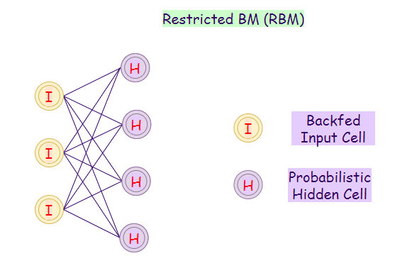
15. Restricted Boltzmann Machine (RBM):

RBMs are a variant of BMs. In this model, neurons in the input layer and the hidden layer may have symmetric connections between them. One thing to notice is that there are no internal connections inside each layer. By contrast, Boltzmann machines may have internal connections in the hidden layer. These restrictions in BMs allow efficient training for the model.

Applications:

• Filtering.
• Feature Learning.
• Classification.
• Risk Detection.
• Business and Economic analysis.

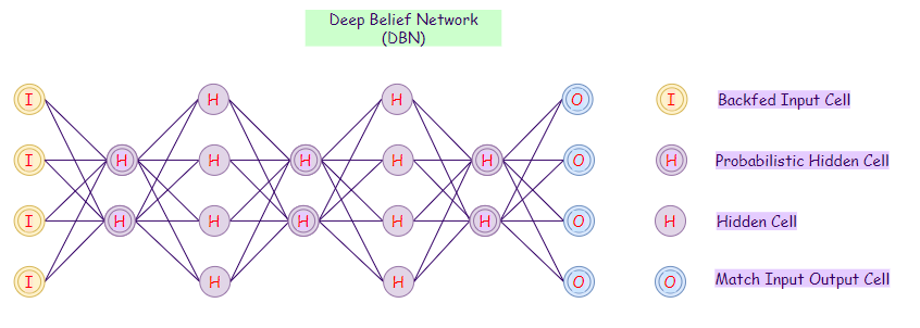
16. Deep Belief Network (DBN):

Deep Belief Networks contain many hidden layers. We can call DBNs with an unsupervised algorithm as it first learns without any supervision. The layers in a DBN acts as a feature detector. After unsupervised training, we can train our model with supervision methods to perform classification. We could represent DBNs as a composition of Restricted Boltzmann Machines (RBM) and Autoencoders (AE), last DBNs use a probabilistic approach toward its results.

Applications:

• Retrieval of Documents/ Images.
• Non-linear Dimensionality Reduction.

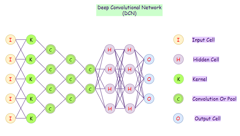
17. Deep Convolutional Network (DCN):

Convolutional Neural Networks are neural networks used primarily for classification of images, clustering of images and object recognition. DNNs enable unsupervised construction of hierarchical image representations. DNNs are used to add much more complex features to it so that it can perform the task with better accuracy.

Applications:

• Identify Faces, Street Signs, Tumors.
• Image Recognition.
• Video Analysis.
• NLP.
• Anomaly Detection.
• Drug Discovery.
• Checkers Game.
• Time Series Forecasting.

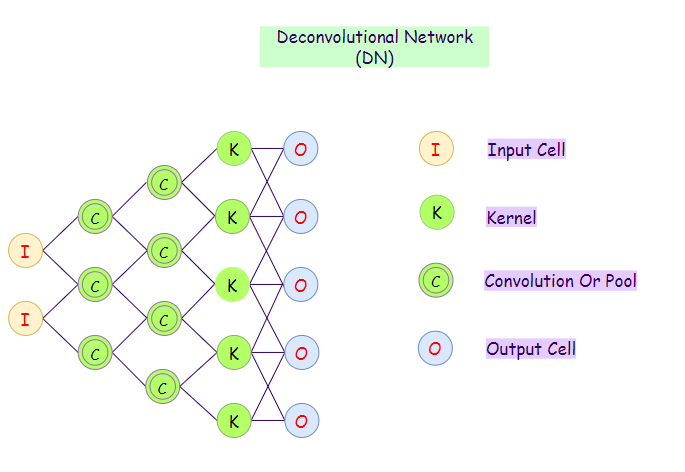
18. Deconvolutional Neural Networks (DN):

Deconvolutional networks are convolutional neural networks (CNNs) that work in a reversed process. Even though a DN is similar to a CNN in nature of work, its application in AI is very different. Deconvolutional networks help in finding lost features or signals in networks that deem useful before. A DN may lose a signal due to having been convoluted with other signals. A Deconvolutional network can take a vector and make a picture out of it.

Applications:

• Image super-resolution.
• Surface depth estimation from an image.
• Optical flow estimation.

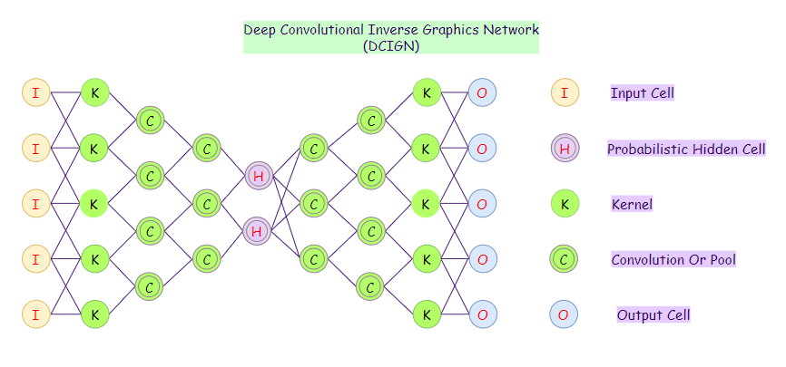
19. Deep Convolutional Inverse Graphics Network (DC-IGN):

Deep Convolutional Inverse Graphics Networks (DC-IGN) aim at relating graphics representations to images. It uses elements like lighting, object location, texture, and other aspects of image design for very sophisticated image processing. It uses various layers to process input and output. The deep convolutional inverse graphics network uses initial layers to encode through various convolutions, utilizing max pooling, and then uses subsequent layers to decode with unspooling.

Applications:

• Manipulation of human faces.

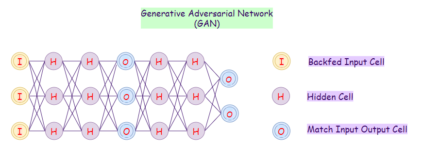
20. Generative Adversarial Network (GAN):

Given training data, GANs learn to generate new data with the same statistics as the training data. For example, if we train our GAN model on photographs, then a trained model will be able to generate new photographs that look authentic to the human eye. The objective of GANs is to distinguish between real and synthetic results so that it can generate more authentic results.

Applications:

• Generate New Human Poses.
• Photos to Emojis.
• Face Aging.
• Super Resolution.
• Clothing Translation.
• Video Prediction.

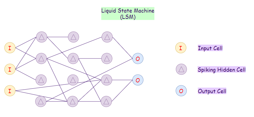
21. Liquid State Machine (LSM) :

A Liquid State Machine (LSM) is a particular kind of spiking neural network. An LSM consists of an extensive collection of neurons. Here each node receives inputs from an external source and other nodes, which can vary by time. Notice that the nodes on LSMs randomly connect to each other. In LSMs, activation functions are replaced by threshold levels. Only when LSMs reach the threshold level, a particular neuron emits its output.

Applications:

• Speech Recognition.
• Computer Vision.

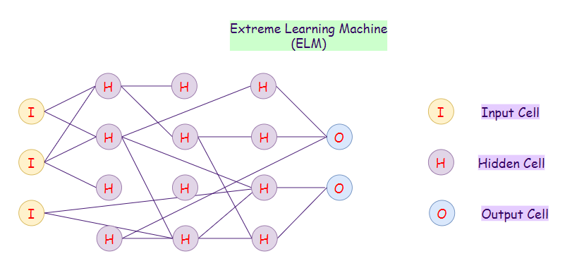
22. Extreme Learning Machine (ELM):

The major drawbacks of conventional systems for more massive datasets are:

• The slow learning speed based on gradient algorithms.
• Tuning all the parameters iteratively.

ELMs randomly choose hidden nodes, and then analytically determines the output weights. Therefore, these algorithms work way faster than the general neural network algorithms. Also, on extreme learning machine networks, randomly assigned weights are generally never updated. ELMs learn the output weights in only one step.

Applications:

• Classification.
• Regression.
• Clustering.
• Sparse Approximation.
• Feature Learning.

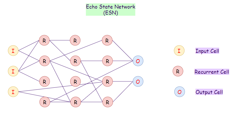
23. Echo State Network (ESN):

The Echo State Network (ESN) is a subtype of recurrent neural networks. Here each input node receives a non-linear signal. In ESN, the hidden nodes are sparsely connected. The connectivity and weights of hidden nodes are randomly assigned. On ESNs, the final output weights are trainable and can be updated.

Applications:

• Timeseries Prediction.
• Data Mining.

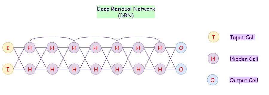
24. Deep Residual Network (DRN):

Deep neural networks with many layers can be tough to train and take much time during the training phase. It may also lead to the degradation of results. Deep Residual Networks (DRNs) prevent degradation of results, even though they have many layers. With DRNs, some parts of its inputs pass to the next layer. Therefore, these networks can be quite deep (It may contain around 300 layers).

Applications:

• Image Classification.
• Object Detection.
• Semantic Segmentation.
• Speech Recognition.
• Language Recognition.

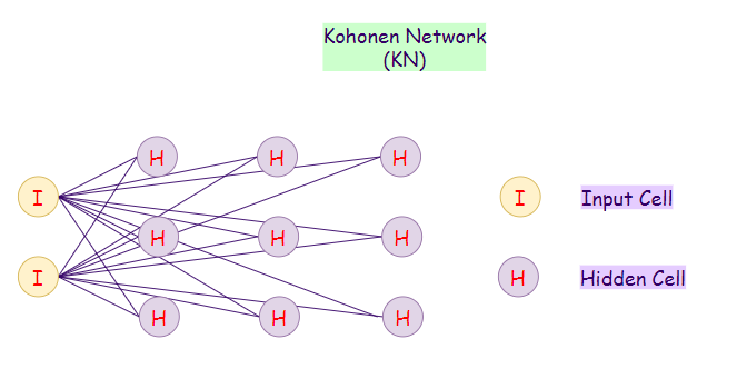
25. Kohonen Networks (KN):

A Kohonen network is an unsupervised algorithm. Kohonen Network is also known as self-organizing maps, which is very useful when we have our data scattered in many dimensions, and we want it in one or two dimensions only. It can be thought of as a method of dimensionality reduction. We use Kohonen networks for visualizing high dimensional data. They use competitive learning rather than error correction learning.

Various Topologies:

• Rectangular Grid Topology.
• Hexagonal Grid Topology.

Applications:

• Dimensionality Reduction.
• Assessment and Prediction of Water Quality.
• Coastal Water Management.

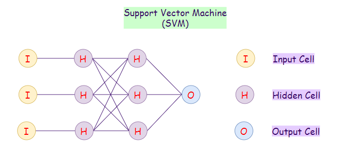
26. Support Vector Machines (SVM):

The Support Vector Machines neural network is a hybrid algorithm of support vector machines and neural networks. For a new set of examples, it always tries to classify them into two categories Yes or No (1 or 0). SVMs are generally used for binary classifications. These are not generally considered as neural networks.

Applications:

• Face Detection.
• Text Categorization.
• Classification.
• Bioinformatics.
• Handwriting recognition.

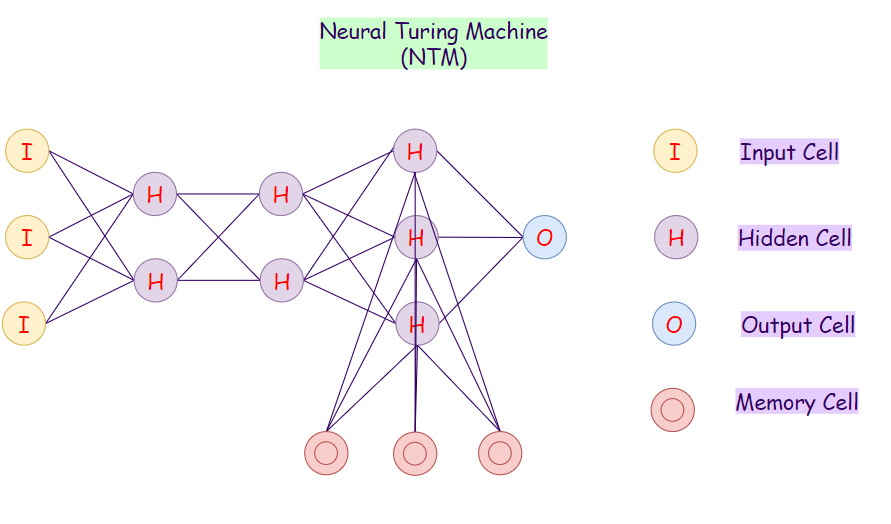
27. Neural Turing Machine (NTM):

A Neural Turing Machine (NTM) architecture contains two primary components:

• Neural Network Controller.
• Memory Bank.

In this neural network, the controller interacts with the external world via input and output vectors. It also performs selective read and write R/W operations by interacting with the memory matrix. A Turing machine is said to be computationally equivalent to a modern computer. Therefore, NTMs extend the capabilities of standard neural networks by interacting with external memory.

Applications:

• Robotics.
• Building an artificial human brain.

We hope you enjoyed this overview of the main types of neural networks. If you have any feedback or if there is something that may need to be revised or revisited, please let us know in the comments or by sending us an email at [email protected].

📚 Check out an overview of machine learning algorithms for beginners with code examples in Python 📚

Terms of Use: This work is a derivative work licensed under a Creative Commons Attribution 4.0 International License. The original referenced graph is attributed to Stefan Leijnen and Fjodor van Veen, which can be found at Research Gate.

DISCLAIMER: The views expressed in this article are those of the author(s) and do not represent the views of Carnegie Mellon University. These writings do not intend to be final products, yet rather a reflection of current thinking, along with being a catalyst for discussion and improvement.

Published via Towards AI

Recommended Articles

I. Best Datasets for Machine Learning and Data Science
II. AI Salaries Heading Skyward
III. What is Machine Learning?
IV. Best Masters Programs in Machine Learning (ML) for 2020
V. Best Ph.D. Programs in Machine Learning (ML) for 2020
VI. Best Machine Learning Blogs
VII. Key Machine Learning Definitions
VIII. Breaking Captcha with Machine Learning in 0.05 Seconds
IX. Machine Learning vs. AI and their Important Differences
X. Ensuring Success Starting a Career in Machine Learning (ML)
XI. Machine Learning Algorithms for Beginners
XII. Neural Networks from Scratch with Python Code and Math in Detail
XIII. Building Neural Networks with Python
XIV. Main Types of Neural Networks
XV. Monte Carlo Simulation Tutorial with Python
XVI. Natural Language Processing Tutorial with Python

References:

[1] Activation Function | Wikipedia | https://en.wikipedia.org/wiki/Activation_function

[2] The perceptron: a probabilistic model for information storage and organization in the brain | Frank Rosenblatt | University of Pennsylvania | https://www.ling.upenn.edu/courses/cogs501/Rosenblatt1958.pdf

[3] Frank Rosenblat’s Mark I Perceptron at the Cornell Aeronautical Laboratory. Buffalo, Newyork, 1960 | Instagram, Machine Learning Department at Carnegie Mellon University | https://www.instagram.com/p/Bn_s3bjBA7n/

[4] Backpropagation | Wikipedia | https://en.wikipedia.org/wiki/Backpropagation

[5] The Neural Network Zoo | Stefan Leijnen and Fjodor van Veen | Research Gate | https://www.researchgate.net/publication/341373030_The_Neural_Network_Zoo

[6] Creative Commons License CCBY | https://creativecommons.org/licenses/by/4.0/