


Descriptive Statistics for Data-driven Decision Making with Python
Last Updated on October 21, 2021 by Editorial Team
This article provides a sample of our book: “Descriptive statistics for data-driven decision making with Python”
Author(s): Pratik Shukla, Roberto Iriondo
Data science and machine learning are scientific disciplines that are ruled by programming and mathematics. Nowadays, most corporations globally generate immense amounts of data that can be further analyzed and visualized by experts to understand trends and forecast predictions. For instance, we can only perform accurate data visualization if our data is clear and understandable.
However, organizations’ data is (frequently) too messy to tinker with — therefore, finding structures and important patterns in data is a crucial task for data science. Statistics provides the methods and tools to find hidden structures and patterns in data so that specialists can make predictions from them — making statistics the most fundamental step in the data science and machine learning scope. We need statistics to transform observations into information. In machine learning, we use a variety of algorithms for prediction, classification, and clustering. Although, there are many useful libraries available to use that will perform mathematical calculations for us.
Nevertheless, we need to know the math behind each of the algorithms and statistical methods we use because knowing these gives us insights into what we are doing and ultimately find our why behind our data-driven decisions.
This work aims to understand the core concepts that form the base for data science, machine learning, and related analytical fields. Our primary goal is to show our readers how to perform calculations and why we need such a methodology. In this book, we try our best to showcase a few core statistical methods with their theories and code examples with python.
Please note that in some cases, the output of python programs may vary from the outputs we get by applying the theoretical concepts — the reason behind it is that we will be using python libraries to display outputs, and in some cases, the programmers that created such libraries used different logic to create their methods. Consequently, we consider it crucial to understand the core logic of what we explain in the theoretical concepts because once we understand the concept, it is relatively easy to write pseudocode and code for the task at hand.
“The quiet statisticians have changed our world; not by discovering new facts or technical developments, but by changing the ways that we reason, experiment, and form our opinions…” ~ Ian Hacking
Introduction
In this work, we are going to take a look at the descriptive statistics. However, before going into statistics, it is crucial to know the basic things we will need. First of all, statistics works on data. If there is no data with us, then there is no possible way statistics can work. We use the data to perform various operations on them to make some helpful conclusions out of it.
Nevertheless, sometimes it is impossible to gather data of everyone related to the research. For example: If we want to measure all the humans’ weight on the earth, it will be impossible to get all humans’ data. So that is why we take samples of data and then perform operations on them.
First of all, we will see the population and sample, and then we will discuss a few sampling techniques.
Population and Sample:
In the study of statistics, our primary focus is on data. Let’s see two critical types of datasets:
- Population
- Sample
The main difference between population and sample can be viewed by the number of observations in each dataset.
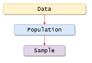
Population includes all the elements or observations that are related to our study. The population is usually denoted with (N), and the numbers we obtain while working with the population are called parameters.
The sample includes one or more observations from the population. Samples are usually denoted with (n), and the
numbers obtained by working with samples are called statistics. Now there are several methods to derive samples from the population. In this book, we are going to see a few of them.
Sampling Techniques:
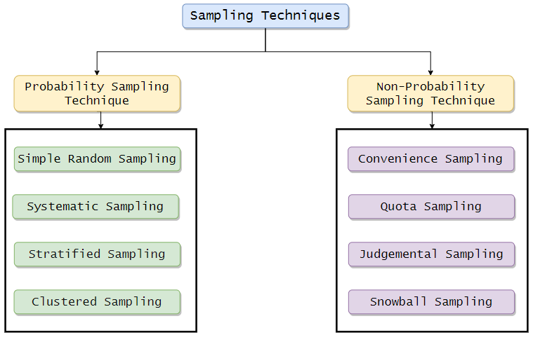
Probability Sampling Techniques:
When each subject or entity has an equal, non-zero chance of getting selected for a sample, it is called the probability Sampling Technique. These samples usually represent a larger population. They provide credible results as there are low chances of bias in sampling.
Simple Random Sampling
In this method, each individual from the population is chosen pseudorandomly, and each member of the population has an equal probability of being selected. In other ways, we can say each member from the entire population has an equal chance of being selected. A simple random sample will be an unbiased representation of the entire population.
For instance:
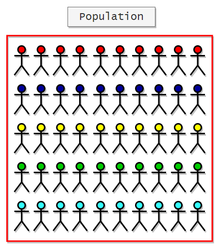
Let’s say we want to choose 10 students from a group of 10000 students randomly. First of all, we need to assign labels to each student. Since there are 10000 students, the labels will start from 0 and end with 9999. Here is a visual representation of labeled students.
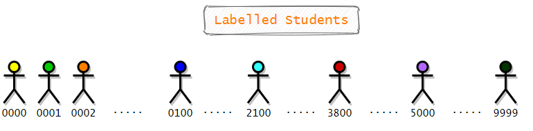
Now we will use simple random sampling to select 10 random students from a total of 10,000 students. To do that, we will use 4 boxes, and each of the boxes will have balls labeled from 0 to 9. Keep in mind that all of the boxes are opaque or non-transparent. So there will be equal chances for each of the students.
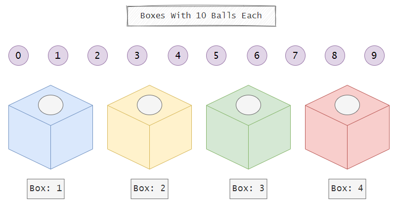
Next, we will call a small child and ask him to draw a ball from each box. Now, we will note down the number printed on the ball. For example, if the child draws a ball labeled as two from the first box, a ball labeled as five from the second box, a ball labeled as nine from the third box, and a ball labeled as 0 from the fourth box, then we will choose the student with the label of 2590.
We will repeat the same process until we have labels for ten students. Hereafter noting down the numbers, the balls will be replaced in their original boxes. So at any point in time, there will be ten balls to choose from. Now here is the list of the students selected by the child.
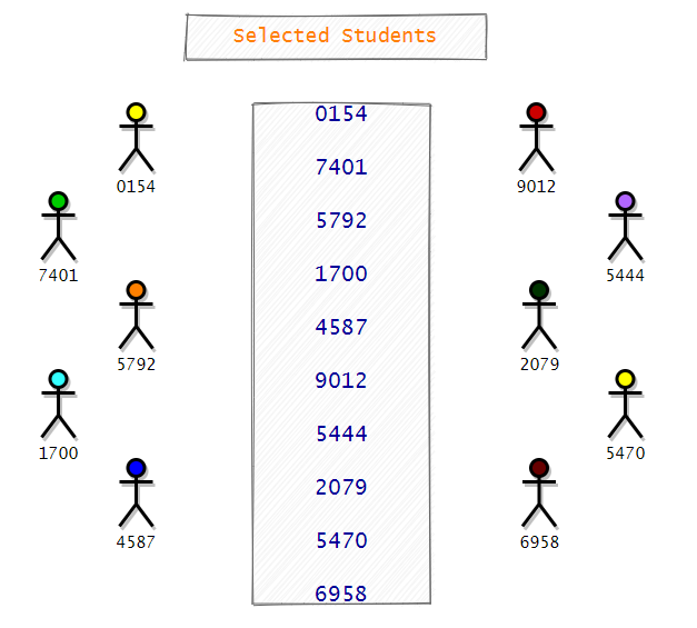
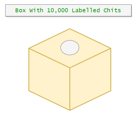
Making this is one way we can choose random students from all of the students. Now notice that in this case, we replaced the balls in their respective boxes. Next, we will see another way we can in which we can implement simple random sampling. However, here we will do it without replacement. So in this method, we will write each number in a chit and put those chits in a single large box, and then we will draw 10 chits from it. Now we do not have to put those chits back in the box. So this is without replacement.
Advantages:
- Simple Random Sampling reduces sampling bias.
- Ease of use.
Disadvantages:
- It requires a little knowledge of the population.
- It may generate sampling errors.
- It is not suitable for a large population.
For example, If we are surveying a population of 10,000 students to find out how many students of them are left-handed. If we take a sample size of 50 students, none of the left-handed students may be selected. So this is a significant disadvantage of this method.
Systematic Sampling
In this method, we are going to select individuals at regular intervals. We can create an interval of any size we want, but it should be suitable for the sample size. It is generally used when the opinions of most people are logically homogeneous.
For instance:
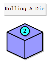
Let’s say we have a population size of 50 students, and we want to select some samples from that. To do that, first of all, we need to decide the start point. We can decide it by rolling a die. Now that we have our start point, it is time to decide the interval. For interval size, we can decide to select every fourth person from the students. Notice that we can take the interval size whatever we want, but it should be per our sample size.
Here we will start with the second student, and after that, we will choose every fourth student. Here is the sample of students selected.
Advantages:
- It is more convenient than simple random sampling.
- It is easy to administer.
Disadvantages:
1. It gives biased results if there are any underlying patterns in the arrangement.
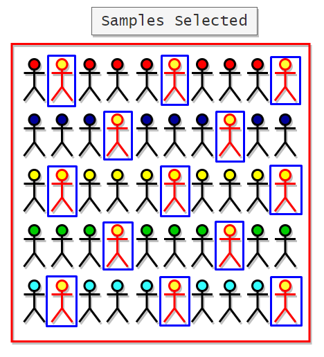
For example, suppose we want to measure the average weight of students. To do that from a population of 50 students, we are going to select some students randomly. Let’s say we selected the students based on our previous calculations.
Here is the representation of selected students:
Here we can see that all the selected students are female. So our sample is biased towards female students. Furthermore, we can say that it will not give us the opinion of the entire population. To get rid of this problem, we can shuffle the population internally before taking samples.
Stratified Sampling
In this method, we will first divide the whole population into groups based on specific characteristics. We generally use this method when we think there will be differences in opinion based on a particular characteristic like age or sex, or race. So what do we do here is we divide the population into subgroups, and then we will use Simple Random Sampling to choose samples from each of these groups. Each of the divided groups is called a Strata. By doing this, we can ensure that we are not overlooking the opinions of a specific group. Let’s take an example to understand it better. Suppose that we want to survey a population on the newly launched game. Here we can think that there can be some opinion differences between groups based on age. So we will divide the population into three groups.
- Children (<18)
- Adults (18+ and <65)
- Elderly (65+)
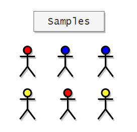
After dividing them into these subgroups, we will use Simple Random Sampling to choose samples from each subgroup.
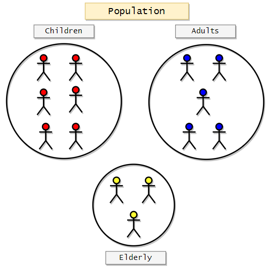
Now that we have divided the population into subgroups, we can use Simple Random Sampling to choose subjects from each group.
Advantages:
1. It improves the accuracy and overall representativeness of the entire population.
Disadvantages:
- It required knowledge of dividing the population-based on specific characteristics.
- It is complex and time-consuming.
Clustered Sampling
In clustered sampling, we use clusters or subgroups to choose samples. Here the clusters are formed naturally. We do not have to create clusters based on specific characteristics.
Let’s take an example to understand it better. Suppose we
want to get information on the weights of people in a particular town. Now consider that town has four streets. So, in this case, our population will be the town or the four streets. Here we can say that we have four subgroups or clusters based on the streets. Now we will choose one cluster from the
4 clusters to gather the required information. So in this method, we know that our population is already divided into four streets. So here, what we can do is we can apply random sampling here to choose one of the four streets from the town, and then we can get information from that street. So we can say that this method runs on top of Simple Random Sampling. Suppose in a town there are four streets.
- Street A
- Street B
- Street C
- Street D
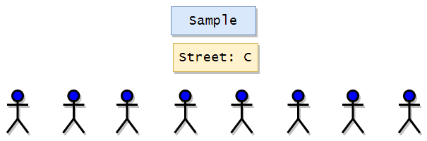
Now we just have to apply Simple Random Sampling to choose 1 out of 4 streets. Here is the visual representation of the technique:
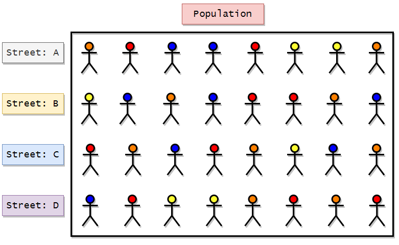
Apply simple random sampling to choose the four streets. Suppose we get street B in our random sampling. Then we can take the necessary information for all people from street B that will represent the entire population.
Advantages:
- If we have a large geographical area, this technique helps a lot because it is easier to get many data from a single cluster than to get a little data from many clusters.
Disadvantages:
- Increased risk of bias.
For example, in the above example, if people in each street are clustered with specific characteristics, this method will give us biased results. If their zodiac signs or race naturally clusters people in this town, this technique will give us biased results.
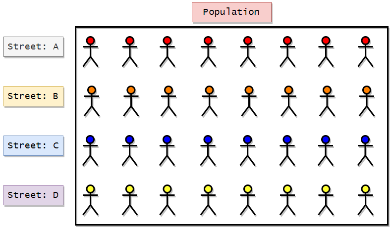
If we apply Simple Random Sampling and if we get street C, then here we can clearly see that the result will be biased and will only represent blue characters.
Non-Probability Sampling Techniques:
In these techniques, the samples or subjects are collected with no specific probability structure in mind. Here we can say that the sampling is not entirely random. The samples are not indeed the representation of the entire population.
Convenience Sampling
Convenience sampling is probably the easiest sampling method because the samples or the participants are selected based on their availability and willingness to participate. In this method, the results are prone to significant bias, and it may
not represent the views of the entire population. One more thing to notice here is that the sample may not represent characteristics like sex or age. It is generally used for preliminary research.
For example:
- Surveying friends.
- Surveying people at the mall.
- Online polls.
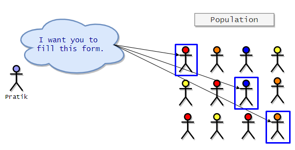
Visual representation of convenience sampling:
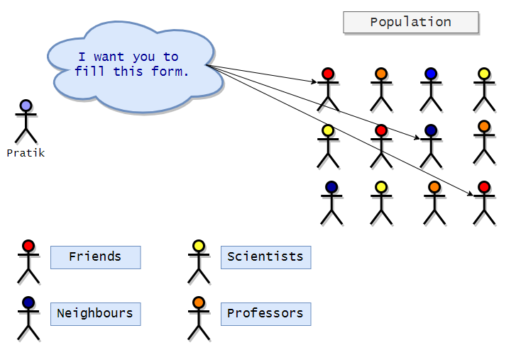
In the representation above, we can see that the researcher (Pratik) chooses his friends and neighbors as subjects for his research as they are easy to convince or reach.
Advantages:
It is easy and can be generated quickly.
Disadvantages:
It is generally a poor representation of the entire population.
Quota Sampling
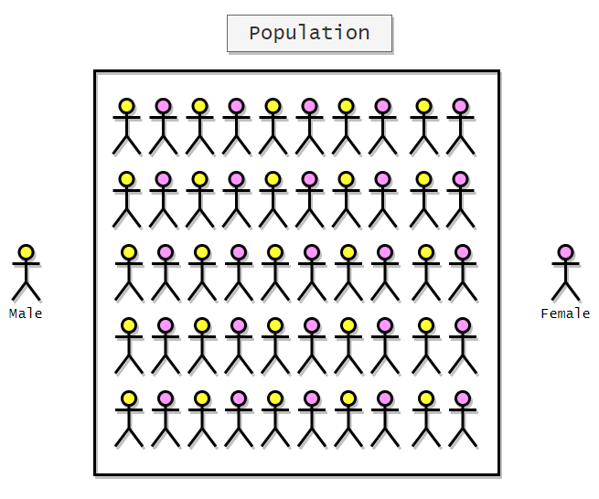
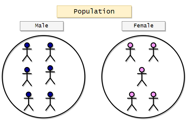
This method is a non-probabilistic approach to stratified sampling. Here we have to divide the whole population into clusters based on some characteristics. After dividing the population into clusters, we can take any person from the groups at our convenience. The subjects will not be chosen randomly. We can also initially fix a quota value to choose the desired number of subjects from each group. For example, let’s say we want to select some candidates for an interview, and we have to select 10 males and 10 females from the population. So what we can do here is we can cluster the population-based on sex, and then we can choose any 10 male and 10 female at our convenience. There is no randomization in choosing the subjects after clustering. The following is a visualization of the sampling technique discussed:
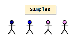
Samples:
Here we are going to choose two candidates from both groups.
Advantages:
- It is straightforward to administer. It is fast and inexpensive.
- We can take into account population proportions if required.
Disadvantages:
- Selection is not random.
Judgemental Sampling
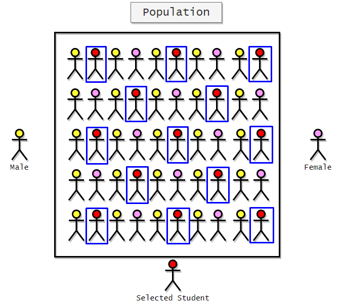
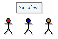
In this method, the researcher chooses his subjects or participants based on his judgment or guts. The researcher can specifically choose a group of people with specific characteristics. The researcher may only choose female participants. So we can say that this method can be biased based on the researcher’s judgment. Using this method, the researchers can choose only those subjects that he/she deems to be a perfect fit for his/her research. It may not represent the opinion of the entire population.
Here is a visualization of the technique discussed.
Samples
Advantages:
- It is time and cost-effective.
Disadvantages:
- The results can be biased.
Snowball Sampling
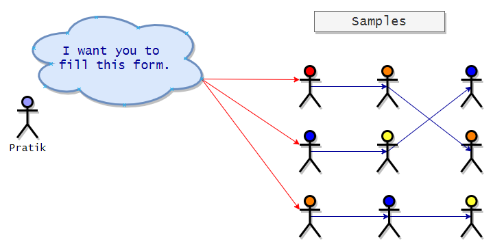
It is a non-probabilistic technique where existing subjects are asked to nominate other subjects best known to them. Here the sample size will grow like a rolling snowball. That is why it is called snowball sampling. Here the existing subjects will recruit other subjects, and the cycle will go on. It is generally used in social-science surveys where subjects with particular characteristics are hard to find. In the following visualization, we can see that initially, Pratik has three subjects, and then the subjects recruit others and so on.
Advantages:
- It is instrumental when the samples are hard to find.
- Low cost.
- Very relevant samples to our study.
Disadvantages:
- This method depends on subjects recruiting other subjects, so there is a high chance of selection bias.
It only works if subjects have other relevant connections.
What is statistics?
According to Wikipedia, statistics is a discipline that concerns the collection, organization, analysis, interpretation, and presentation of data. We can also say that statistics is a science of collecting and analyzing numerical data in large quantities. We can also say that statistics is a matter of science and logic.
Importance of statistics in Data Science and Machine Learning
Data science and machine learning are scientific disciplines that are dominated by programming and mathematics. Most data-corporations in the world generate vast amounts of data that experts can further analyze and visualize to understand the trends. Data visualization can only be performed if the data is clear and understandable. However, the data generated by
organizations are too messy to handle. So we can say that finding structures and basic patterns in data is an essential task for data science. Statistics provides the methods and tools to find the hidden structures and patterns in the data so that experts can make predictions from them. Statistics is the fundamental step in the Data Science world. We can say we need statistics to transform observations into information. In machine learning, we use various kinds of algorithms for prediction, classification, and clustering. However, there are many useful libraries available for use that will perform mathematical calculations for us. Nevertheless, it is vital to know the math behind each of the algorithms because it provides insights into what we are doing and why?
Instead of applying cool-sounding machine learning algorithms to our data to make predictions, it is imperative to understand the pattern to know the data’s distribution. Now how will the distribution of data help us? After knowing the distribution of data, we can look at the limitations of machine learning algorithms and apply them to give us the best results. In our projects, we use a part of data to train the algorithm and make predictions from it. To train the model for our algorithm, we generally use the Python programming language.
Moreover, we are well aware that python is relatively slower than other programming languages. However, the simple syntax and well-developed libraries give programmers a reason to lean towards it. In the real world, the data will be in large quantities, so here we cannot take the risk of training our model based on an algorithm that provides no useful insights. That is why it is essential to understand the distribution of data. In future work, we will show the different types of distributions of data.
Types of Statistics:
Statistics can be divided into two main categories.
- Descriptive Statistics
- Inferential Statistics
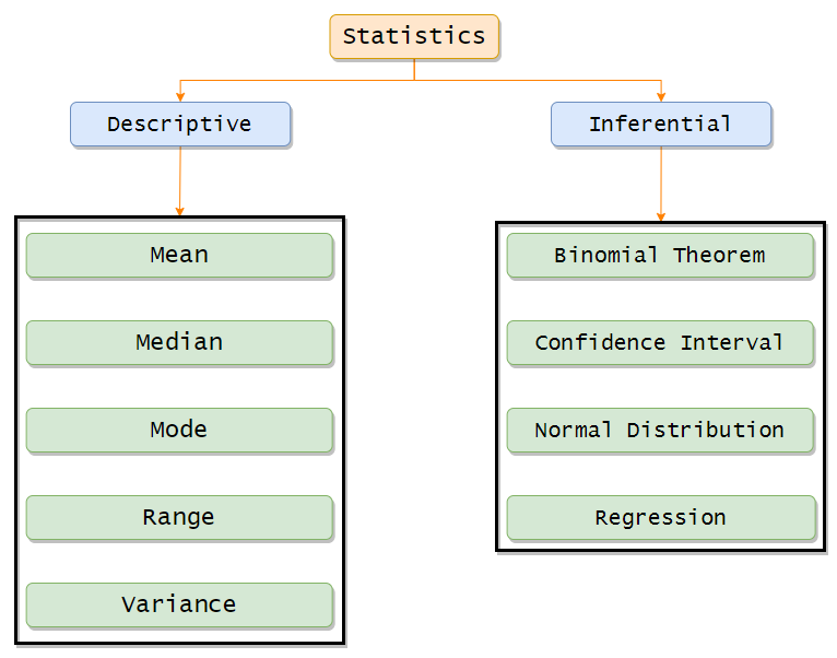
Descriptive Statistics:
Descriptive statistics fundamentally works on organizing and summarizing data using graphs. We can summarize the data and visualize it using Bar graphs, Histograms, and Pie charts.
We can also view the shape and skewness of the graphs. Descriptive statistics include measures to find central tendency values like mean, median, and mode. Other than that, we can also find the measure of variability or the spread of data with the range, variance, and standard deviation values.
Inferential Statistics:
In inferential statistics, we use the sample data to make an inference or draw the population’s conclusion. It uses probability to find out the confidence of the predictions we make.
In this work, we will mainly focus on Descriptive Statistics.
Measure of Central Tendency:
Central tendency refers to an idea that suggests one number that best summarizes our whole dataset. It may also be called the center of the distribution.
Arithmetic Mean:
Mean can be referred to as a central tendency of the data. It is a single number around which our data is spread around. In short, we can say that it is a single number that best represents the whole dataset.
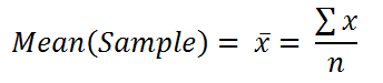
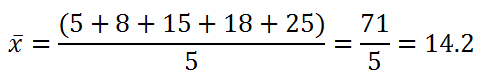
The mean or average of a dataset is found by adding all the numbers in it and then dividing the sum by the dataset’s length.
Formula of the mean for population:
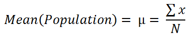
Formula of the mean for sample:
Example:
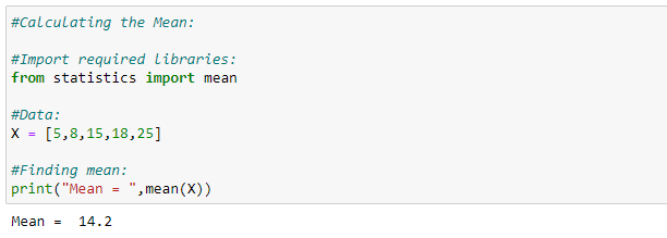
- Find the mean for the following dataset: [5, 8, 15, 18, 25]
Python implementation:
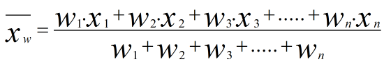
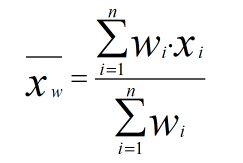
Weighted Mean:
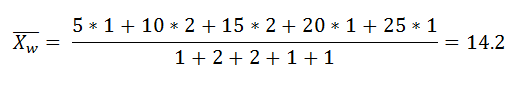
When we have the same numbers many times in some data, then to find the mean instead of simply adding it up and then dividing by its length, we will find the weighted frequency for each number so that our process will become faster.
Find the weighted mean for the following data:
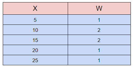
Python implementation:

Mean for Categorical Dataset:
Let’s say we went to a pet show that only has dogs and cats. As we move forward, we are noting whether the pet is a dog or cat. The following is the final observation or data.
[Dog, Cat, Cat, Dog, Cat, Cat, Dog, Cat, Cat, Dog]
Now we want to find the mean of this categorical dataset. To do that, we have to convert the categorical dataset into a numerical dataset. Here we are denoting cat as 0 and Dog as
1. Hence, here is our numerical dataset.
[1,0,0,1,0,0,1,0,0,1]
Now we can apply our regular mean formula:
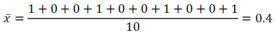
Now here we can see that the mean is centered towards 0. Therefore, in our dataset, the number of cats is higher than the number of dogs.
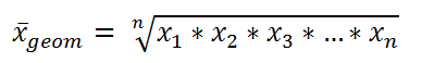
Geometric Mean:
The geometric mean is the “nth” root when we multiply n numbers.
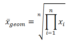
In a simplified way:
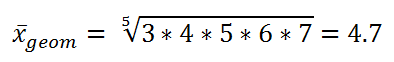
Example:
Find the geometric mean of [3, 4, 5, 6, 7].
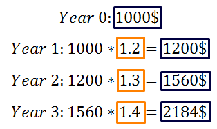
Use-case:
It is generally used when we are trying to calculate the average growth rate where the growth is determined by multiplication, not addition.
For example:
My Apple stock gained 20% in year 1, 30% in year 2, and 40% in year 3. Then what is the average yearly rate of return?
DISCLAIMER: The views expressed in this work are those of the author(s) and do not represent the views of any company (directly or indirectly) associated with the author(s). This book does not intend to be a final product, yet rather a reflection of current thinking along with being a catalyst for discussion and improvement.
All images are from the author(s) unless stated otherwise.
Published via Towards AI
Resources:
References:
- All the puns and jokes on statistics are referenced from, Statistics and Statisticians, “Science Jokes:1. MATHEMATICS: 1.2 STATISTICS AND STATISTICIANS”. 2021. Jcdverha.Home.Xs4all.Nl. https://jcdverha.home.xs4all.nl/scijokes/1_2.html.
- “Percentiles And Quartiles”. 2021. Statisticslectures.Com. http://www.statisticslectures.com/topics/percentilequartile/.
- 2021. Coursehero.Com. https://www.coursehero.com/file/p3b7kgk/The-variance-is-a-weighted-average-of-the-squared-deviations-from-the-mean/.
- “Normal Distribution Of Data”. 2021. Varsitytutors.Com. https://www.varsitytutors.com/hotmath/hotmath_help/topics/normal-distribution-of-data.
- “Skewness”. 2021. En.Wikipedia.Org. https://en.wikipedia.org/wiki/Skewness.
- “Let Us Understand The Correlation Matrix And Covariance Matrix”. 2020. Medium. https://towardsdatascience.com/let-us-understand-the-correlation-matrix-and-covariance-matrix-d42e6b643c22.
- “Covariance Vs Correlation | Difference Between Correlation And Covariance”. 2020. Greatlearning Blog: Free Resources What Matters To Shape Your Career!. https://www.mygreatlearning.com/blog/covariance-vs-correlation/.
- “Moment (Mathematics)”. 2021. En.Wikipedia.Org. https://en.wikipedia.org/wiki/Moment_(mathematics).
- “Confidence Interval Definition”. 2021. Investopedia. https://www.investopedia.com/terms/c/confidenceinterval.asp.
- “Normal Distribution”. 2021. En.Wikipedia.Org. https://en.wikipedia.org/wiki/Normal_distribution.
- “Kurtosis”. 2021. En.Wikipedia.Org. https://en.wikipedia.org/wiki/Kurtosis.
- All the diagrams were made using, “Flowchart Maker & Online Diagram Software”. 2021. App.Diagrams.Net. https://app.diagrams.net/.
Towards AI Academy
We Build Enterprise-Grade AI. We'll Teach You to Master It Too.
15 engineers. 100,000+ students. Towards AI Academy teaches what actually survives production.
Start free — no commitment:
→ 6-Day Agentic AI Engineering Email Guide — one practical lesson per day
→ Agents Architecture Cheatsheet — 3 years of architecture decisions in 6 pages
Our courses:
→ AI Engineering Certification — 90+ lessons from project selection to deployed product. The most comprehensive practical LLM course out there.
→ Agent Engineering Course — Hands on with production agent architectures, memory, routing, and eval frameworks — built from real enterprise engagements.
→ AI for Work — Understand, evaluate, and apply AI for complex work tasks.
Note: Article content contains the views of the contributing authors and not Towards AI.
Related posts


Recent Posts
")


")


