The Gradient Descent Algorithm

Author(s): Towards AI Editorial Team

Originally published on Towards AI the World’s Leading AI and Technology News and Media Company. If you are building an AI-related product or service, we invite you to consider becoming an AI sponsor. At Towards AI, we help scale AI and technology startups. Let us help you unleash your technology to the masses.

The What, Why, and Hows of the Gradient Descent Algorithm

Author(s): Pratik Shukla

“The cure for boredom is curiosity. There is no cure for curiosity.” — Dorothy Parker

The Gradient Descent Series of Blogs:

1. The Gradient Descent Algorithm (You are here!)
2. Mathematical Intuition behind the Gradient Descent Algorithm
3. The Gradient Descent Algorithm & its Variants

Table of Contents:

1. Motivation for the Gradient Descent Series
2. What is the gradient descent algorithm?
3. The intuition behind the gradient descent algorithm
4. Why do we need the gradient descent algorithm?
5. How does the gradient descent algorithm work?
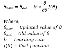
6. The formula of the gradient descent algorithm
7. Why do we use gradients?
8. A brief introduction to the directional derivatives
9. What is the direction of the steepest ascent?
10. An example proving the direction of the steepest ascent
11. An explanation of the ( — ) sign in the gradient descent algorithm
12. Why learning rate?
13. Some basic rules of differentiation
14. Gradient descent algorithm for one variable
15. Gradient descent algorithm for two variables
16. Conclusion
17. References and Resources

Motivation for the Gradient Descent Series:

We are pleased to introduce our first blog series on machine learning algorithms! We want to educate our readers on the fundamental principles behind machine learning algorithms. Nowadays, one of the numerous Python packages can be used to implement most machine-learning algorithms. We can quickly implement any machine learning method using these Python packages in only a few minutes. We find it intriguing, don’t you? However, many students and professionals struggle when they need to make changes to the algorithm. To understand how machine learning algorithms function at their core, we have developed this series of blogs. We intend to provide a short series on more machine learning algorithms in the future, and we hope you will find this one exciting and valuable!

Optimization is at the core of machine learning — it’s a big part of what makes an algorithm’s results “good” in the ways we want them to be. Many machine learning algorithms find the optimal values of their parameters using the gradient descent algorithm. Therefore, understanding the gradient descent algorithm is essential to understanding how AI produces good results.

In the first part of this series, we will provide a strong background on the gradient descent algorithm’s what, why, and hows. In the second part, we will offer you a robust mathematical intuition on how the gradient descent algorithm finds the best values of its parameters. In the last part of the series, we will compare the variants of the gradient descent algorithm with their elaborated code examples in Python. This series is intended for beginners and experts alike — come one, come all!

What is the Gradient Descent Algorithm?

Wikipedia formally defines the phrase gradient descent as follows:

In mathematics, gradient descent is a first-order iterative optimization algorithm for finding a local minimum of a differentiable function.

Gradient descent is a machine learning algorithm that operates iteratively to find the optimal values for its parameters. The algorithm considers the function’s gradient, the user-defined learning rate, and the initial parameter values while updating the parameter values.

Intuition Behind the Gradient Descent Algorithm:

Let’s use a metaphor to visualize what gradient descent looks like in action. Say that we’re hiking a mountain and unfortunately, it begins to rain while we are in the middle of our hike. Our objective is to descend the mountain as rapidly as possible to seek shelter. So, what will be our strategy for doing this? Remember that we can’t see very far because it’s raining. In all directions around us, we can only perceive the nearby movements.

Here’s what comes to mind. We will scan the area around us in search of a move that will send us down as rapidly as feasible. Once we find that direction, we will take a baby step in that direction. We’ll continue doing this until we get to the bottom of the mountain. So, in essence, this is how the gradient descent method locates the global minimum (the lowest point of the entire set of data we’re analyzing). Here is how we can relate this example to the gradient descent algorithm.

current position → → → initial parameters
baby step → → → learning rate
direction → → → partial derivative (gradient)

Why do We Need the Gradient Descent Algorithm?

In many machine learning models, our ultimate goal is to find the best parameter values that reduce the cost associated with the predictions. To do this, we initially start with random values of these parameters and try to find the optimal ones. To find the optimal values, we use the gradient descent algorithm.

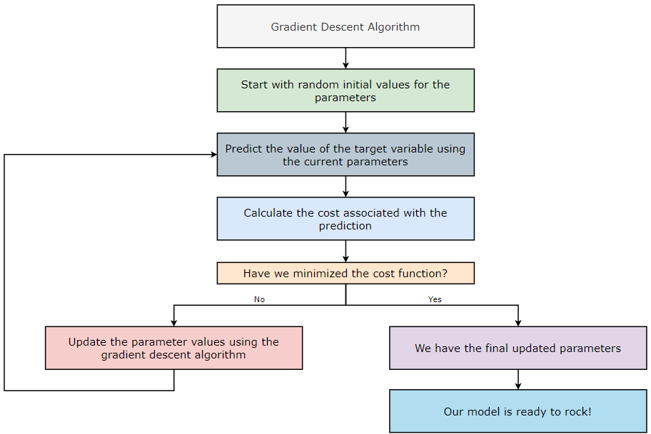
How does the Gradient Descent Algorithm Work?

1. Start with random initial values for the parameters.
2. Predict the value of the target variable using the current parameters.
3. Calculate the cost associated with the prediction.
4. Have we minimized the cost? If yes, then go to step — 6. If no, then go to step — 5.
5. Update the parameter values using the gradient descent algorithm and return to step — 2.
6. We have our final updated parameters.
7. Our model is ready to roll (down the mountain)!

The Formula of the Gradient Descent Algorithm:

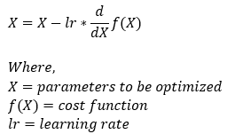
Now, let’s understand the meaning behind each of the terms mentioned in the above formula. Let’s first start by understanding the directional derivatives.

Note: Our ultimate goal is to find the optimal parameters as quickly as possible. So, we will need something to help us move in the right direction as soon as possible.

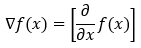
Why do we use gradients?

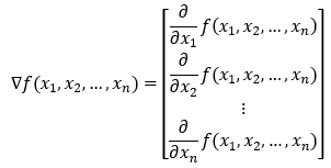
Gradients: Gradients are nothing but a vector whose entries are partial derivatives of a function.

Suppose we have a function f(x) of one variable x. In this case, we will have only one partial derivative. The partial derivative shown in the below image gives us the value of how quickly the function is changing (increasing or decreasing) in the x direction (along the x-axis). We can write the partial derivative in the gradient form as follows.

Let’s say we have a function f(x, y) of two variables, x and y. In this case, we will have two partial derivatives. The partial derivative shown in the below image gives us the value of how quickly the function is changing (increasing or decreasing) in the x direction and y direction (along the x-axis and y-axis). We can write the partial derivative in the gradient form as follows.

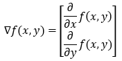
To generalize this, we can have a function with n variables, and its gradient will have n elements.

But now the question is, what if we want to find the derivative in some directions other than just along the axis? We know that we can travel in an infinite number of directions from a given point. Now, to find the gradient in any direction, we will use the concept of directional derivatives.

A Brief Introduction to the Directional Derivatives:

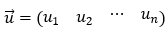
Unit vector: A unit vector is a vector with a magnitude of 1.

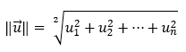
How do we find the length or magnitude of a vector?

Consider the following for a vector u.

The vector’s length is then calculated as the square root of the sum of all its components squared.

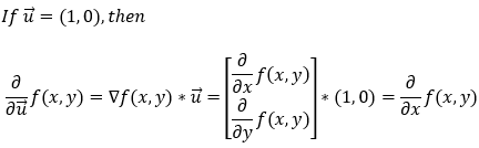
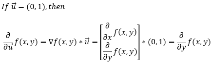
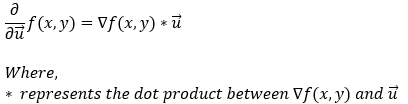
The derivative of a function f(x, y) in the direction of vector u (a unit vector) is given by the dot product of the function’s gradient with the unit vector u. Mathematically, we can represent it in the following form.

The above equation gives us the partial derivative of f(x, y) in any direction. Now, let’s see how it works if we want to find the partial derivative along the x-axis. First, if we want to find the partial derivative in the x direction, the unit vector u will be (1, 0). Now, let’s calculate the partial derivative along the x-axis.

Next, let’s see how it works if we want to find the partial derivative along the y-axis. First of all, if we want to find the partial derivative in the y direction, the unit vector u will be (0, 1). Now, let’s calculate the partial derivative along the y-axis.

Note: The length (magnitude) of the unit vector must be 1.

Now that we know how to find the partial derivatives in all directions, we need to find the direction in which the partial derivative gives us the maximum change, because, in our case, we want to find the optimum values as quickly as possible.

What is the direction of the steepest ascent?

As of right now, we are aware that the directional derivatives are shown as follows.

Next, we can replace the dot product between two vectors with the cosine value of the angle between them.

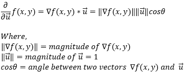
Now, note that since u is a unit vector, its magnitude is always going to be 1.

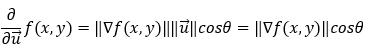
Now, in the above equation, we do not have control over the magnitude of the gradient. We can only control the angle θ. So, to maximize the partial derivative of the function, we need to maximize cosθ. Now, we all know that cosθ is maximized (1) when θ = 0 (cos0 = 1). It means that the value of the derivative is maximized when the angle between the gradient and unit vector is 0. In other words, we can say that the value of the partial derivative is maximized when the unit vector (direction vector) points in the direction of the gradient.

So, in conclusion, we can say that finding the partial derivative in the direction of the gradient gives us the steepest ascent. Now, let’s understand this with the help of an example.

Example proving the direction of the steepest ascent:

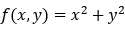
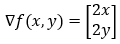
Find the gradient of the function f(x, y) = x² + y² at the point (3, 2).

1. Step — 1:

We have a function f(x, y) of two variables x and y.

2. Step — 2:

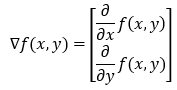
Next, we will find the gradient of the function. Since there are two variables in our function, the gradient vector will have two elements in it.

3. Step — 3:

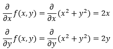
Next, we are calculating the gradient of the function f(x, y) = x² + y².

4. Step — 4:

The gradient of the function can be written as follows.

5. Step — 5:

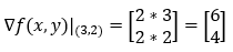
Next, we calculate the gradient of the function at the point (3, 2).

6. Step — 6:

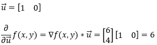
Next, we are finding the partial derivative of the function f(x, y) along the x-axis (1, 0).

7. Step — 7:

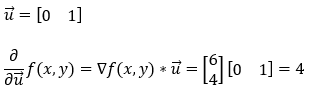
Next, we are finding the partial derivative of the function f(x, y) along the y-axis (0, 1).

8. Step — 8:

Next, we find the partial derivative of the function f(x, y) in the direction of (1, 1). Note that here we will have to take care of the magnitude of the unit vector.

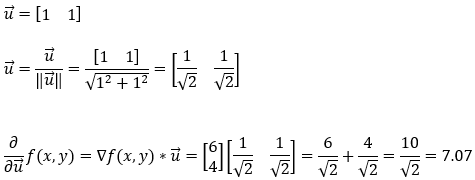
9. Step — 9:

Next, we find the partial derivative of the function f(x, y) in the direction of the gradient (3, 2). Please note that this is the direction of the gradient vector. Also, here we will have to take care of the magnitude of the unit vector.

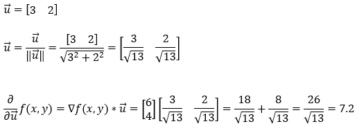
10. Step — 10:

So, based on the calculations shown in Step — 6, Step — 7, Step — 8, Step — 9, we can confidently say that the direction of the steepest ascent is the direction of the gradient.

In the gradient descent algorithm, we aim to find the optimal parameters as quickly as possible. So, this is the reason why we use the partial derivatives in the gradient descent algorithm.

But wait… there is a catch!

In the gradient descent algorithm, we want to find the minimum point. However, using the gradient will lead us to the highest point because it gives us the steepest ascent. So, what do we about it?

Explanation for the ( — ) sign in the gradient descent algorithm:

Now, we know that the gradient gives us the steepest ascent. So, if we proceed in the direction of the steepest ascent, we will never reach the minimum point. Our ultimate goal is to quickly find a way to reach the minimum point. So, to go in the direction of the steepest descent, we will travel in the exact opposite direction of the steepest ascent. This is the reason why we use the ( — ) sign.

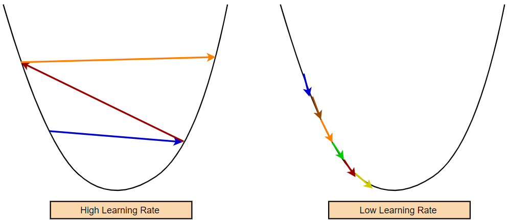
Why Learning Rate?

Please be aware that we have no control over the gradient’s magnitude. Occasionally we may get a very high gradient value. Therefore, if we don’t somehow manage to slow down the rate of change, we’ll end up making some very huge strides. It is important to remember that a high learning rate may only provide us with sub-optimal parameter values. In contrast, a lower learning rate may necessitate more training epochs to obtain the optimal value.

The gradient descent approach has a hyperparameter that regulates how quickly our model learns new information. This hyperparameter is known as the learning rate. Our model’s learning rate determines how quickly parameter values are changed. We must set the learning rate at an optimum value. If the learning rate is too high, our model might take big steps and miss the minimum. So, a higher learning rate may result in the non-convergence of the model. On the other hand, if the learning is too small, the model will take too much time to converge.

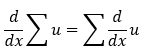
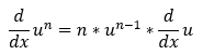
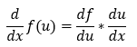
Some Basic Rules of Differentiation:

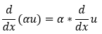
1. Scalar multiplication rule:

2. The summation rule:

3. The power rule:

4. The chain rule:

Now, let’s take a couple of examples to understand how the gradient descent algorithm works.

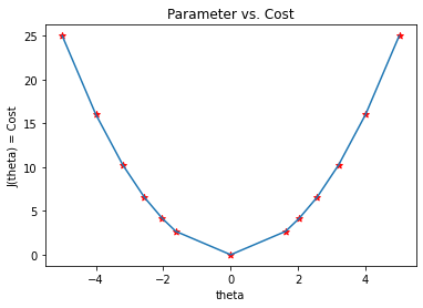
Gradient descent for one variable:

Let’s start off with a very simple cost function. Let’s say we have a cost function (J(θ) = θ²) involving only one parameter (θ), and our goal is to find the optimal value of the parameter (θ) such that it minimizes the cost function (J(θ) = θ²).

From our cost function (J(θ) = θ²), we can clearly say that it will be minimum at θ=0. However, deriving such conclusions will not be easy while we are working with more complex functions. To do that, we will use the gradient descent algorithm. Let’s see how we can apply the gradient descent algorithm to find the optimal value of the parameter (θ).

1. Step — 1:

Our cost function with one parameter (θ) is given by,

2. Step — 2:

Our ultimate goal is to minimize the cost function by finding the optimal value of parameter θ.

3. Step — 3:

The formula for the gradient descent algorithm is the following.

4. Step — 4:

To ease the calculations, we are considering the learning rate of 0.1.

5. Step — 5:

Next, we find the partial derivative of the cost function.

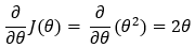
6. Step — 6:

Next, we use the partial derivative of Step — 5 and substitute it into the formula given in Step — 3.

7. Step — 7:

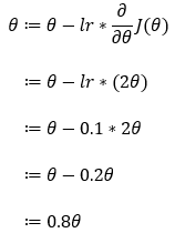
Now, let’s understand how the gradient descent algorithm works with the help of an example. Here, we are starting with the value of θ=5, and we will find the optimal value for θ such that it minimizes the cost function. Next, we will also begin with the value of θ=-5 to check whether it can find the optimal values for the cost function or not. Please note that here we are using the above-derived gradient descent rule to update the value of the parameter θ.

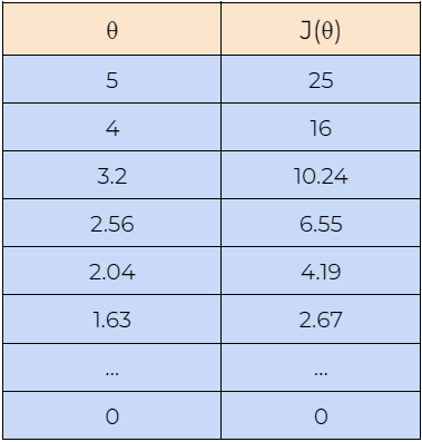
8. Step — 8:

Next, we plot the graph of the data shown in the above tables. We can see in the graph that the gradient descent algorithm is able to find the optimal value of θ and minimizes the cost function J(θ).

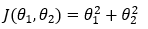
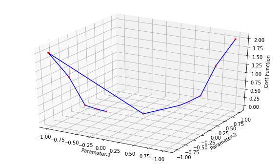
Gradient Descent for two variables:

Now, let’s move on to the cost function with two variables and see how it goes.

1. Step — 1:

Our cost function with two parameters (θ1 and θ2) is given by,

2. Step — 2:

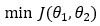
Our ultimate goal is to minimize the cost function by finding the optimal value of parameters θ1 and θ2.

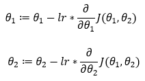
3. Step — 3:

The formula for the gradient descent algorithm is as follows.

4. Step — 4:

We will use the formula given in Step — 3 to find the optimal values of our parameters θ1 and θ2.

4. Step — 4:

Next, we find the partial derivatives of the cost functions with respect to the parameters θ1 and θ2.

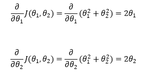
5. Step — 5:

Next, we are using the partial derivatives derived in Step — 4 to substitute in Step — 3.

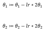
6. Step — 6:

To simplify the calculations, we are going to use the learning rate of 0.1.

7. Step — 7:

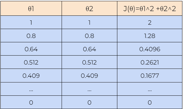
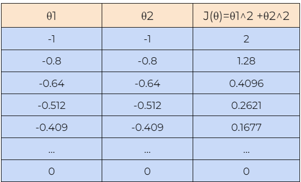
Now, let’s understand how the gradient descent algorithm works with the help of an example. Here, we are starting with the value of θ1=1 and θ2=1, and we will find the optimal value for θ1 and θ2 such that it minimizes the cost function. Next, we will also start with the value of θ1=-1 and θ2=-1 to check whether the gradient descent algorithm can find the optimal values for the cost function or not.

8. Step — 8:

Next, we plot the graph of the data shown in the above tables. We can see in the graph that the gradient descent algorithm is able to find the optimal values of θ1 and θ2 and minimizes the cost function J(θ).

Conclusion:

There you have it! We’ve gone over the basics of the gradient descent algorithm and its important role in machine learning. Feel free to go over any of the calculations or concepts that might not be clear on the first pass-over. Now that you’ve successfully learned how to descend the mountain, learn about the other ways gradient descent can help solve problems in the next installment of the Gradient Descent series.

Citation:

For attribution in academic contexts, please cite this work as:

Shukla, et al., “The Gradient Descent Algorithm”, Towards AI, 2022

BibTex Citation:

@article{pratik_2022, 
 title={The Gradient Descent Algorithm}, 
 url={https://towardsai.net/neural-networks-with-python}, 
 journal={Towards AI}, 
 publisher={Towards AI Co.}, 
 author={Pratik, Shukla},
 editor={Lauren, Keegan},  
 year={2022}, 
 month={Oct}
}

References and Resources:

1. Gradient descent — Wikipedia

---

The Gradient Descent Algorithm was originally published in Towards AI on Medium, where people are continuing the conversation by highlighting and responding to this story.

Join thousands of data leaders on the AI newsletter. It’s free, we don’t spam, and we never share your email address. Keep up to date with the latest work in AI. From research to projects and ideas. If you are building an AI startup, an AI-related product, or a service, we invite you to consider becoming a sponsor.

Published via Towards AI