


The Gradient Descent Algorithm and its Variants
Last Updated on October 25, 2022 by Editorial Team
Author(s): Towards AI Editorial Team
Originally published on Towards AI the World’s Leading AI and Technology News and Media Company. If you are building an AI-related product or service, we invite you to consider becoming an AI sponsor. At Towards AI, we help scale AI and technology startups. Let us help you unleash your technology to the masses.
Gradient Descent Algorithm with Code Examples in Python
Author(s): Pratik Shukla
“Educating the mind without educating the heart is no education at all.” ― Aristotle
The Gradient Descent Series of Blogs:
- The Gradient Descent Algorithm
- Mathematical Intuition behind the Gradient Descent Algorithm
- The Gradient Descent Algorithm & its Variants (You are here!)
Table of contents:
- Introduction
- Batch Gradient Descent (BGD)
- Stochastic Gradient Descent (SGD)
- Mini-Batch Gradient Descent (MBGD)
- Graph Comparison
- End Notes
- Resources
- References
Introduction:
Drumroll, please: Welcome to the finale of the Gradient Descent series! In this blog, we will dive deeper into the gradient descent algorithm. We will discuss all the fun flavors of the gradient descent algorithm along with their code examples in Python. We will also examine the differences between the algorithms based on the number of calculations performed in each algorithm. We’re leaving no stone unturned today, so we request that you run the Google Colab files as you read the document; doing so will give you a more precise understanding of the topic to see it in action. Let’s get into it!
Batch Gradient Descent:
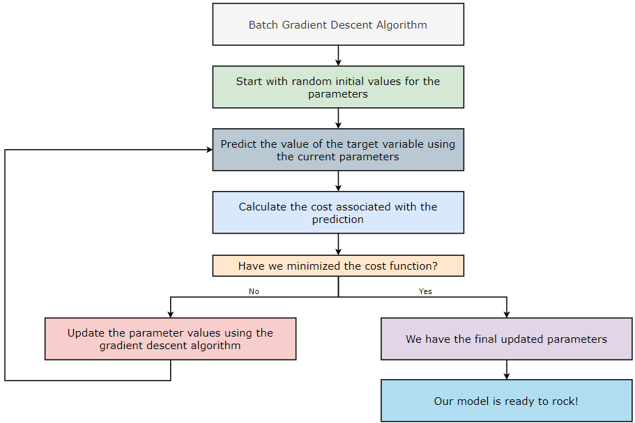
The Batch Gradient Descent (BGD) algorithm considers all the training examples in each iteration. If the dataset contains a large number of training examples and a large number of features, implementing the Batch Gradient Descent (BGD) algorithm becomes computationally expensive — so mind your budget! Let’s take an example to understand it in a better way.
Batch Gradient Descent (BGD):
Number of training examples per iterations = 1 million = 1⁰⁶
Number of iterations = 1000 = 1⁰³
Number of parameters to be trained = 10000 = 1⁰⁴
Total computations = 1⁰⁶ * 1⁰³* 1⁰⁴ = 1⁰¹³
Now, let’s see how the Batch Gradient Descent (BGD) algorithm is implemented.
1. Step — 1:
First, we are downloading the data file from the GitHub repository.
2. Step — 2:
Next, we import some required libraries to read, manipulate, and visualize the data.
3. Step — 3:
Next, we are reading the data file, and then printing the first five rows of it.
4. Step — 4:
Next, we are dividing the dataset into features and target variables.
Dimensions: X = (200, 3) & Y = (200, )
5. Step — 5:
To perform matrix calculations in further steps, we need to reshape the target variable.
Dimensions: X = (200, 3) & Y = (200, 1)
6. Step — 6:
Next, we are normalizing the dataset.
Dimensions: X = (200, 3) & Y = (200, 1)
7. Step — 7:
Next, we are getting the initial values for the bias and weights matrices. We will use these values in the first iteration while performing forward propagation.
Dimensions: bias = (1, 1) & weights = (1, 3)
8. Step — 8:
Next, we perform the forward propagation step. This step is based on the following formula.
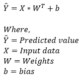
Dimensions: predicted_value = (1, 1)+(200, 3)*(3,1) = (1, 1)+(200, 1) = (200, 1)
9. Step — 9:
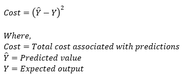
Next, we are going to calculate the cost associated with our prediction. This step is based on the following formula.
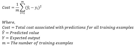
Dimensions: cost = scalar value
10. Step — 10:
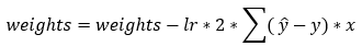
Next, we update the parameter values of weights and bias using the gradient descent algorithm. This step is based on the following formulas. Please note that the reason why we’re not summing over the values of the weights is that our weight matrix is not a 1*1 matrix.
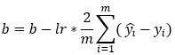
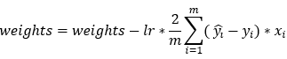
Dimensions: db = sum(200, 1) = (1, 1)
Dimensions: dw = (1, 200) * (200, 3) = (1, 3)
Dimensions: bias = (1, 1) & weights = (1, 3)
11. Step — 11:
Next, we are going to use all the functions we just defined to run the gradient descent algorithm. We are also creating an empty list called cost_list to store the cost values of all the iterations. This list will be put to use to plot a graph in further steps.
12. Step — 12:
Next, we are actually calling the function to get the final results. Please note that we are running the entire code for 200 iterations. Also, here we have specified the learning rate of 0.01.
13. Step — 13:
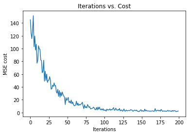
Next, we are plotting the graph of iterations vs. cost.
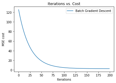
14. Step — 14:
Next, we are printing the final weights values after all the iterations are done.
15. Step — 15:
Next, we print the final bias value after all the iterations are done.
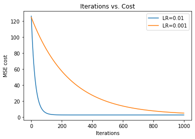
16. Step — 16:
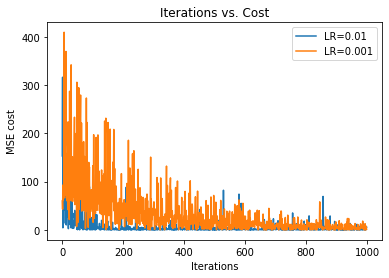
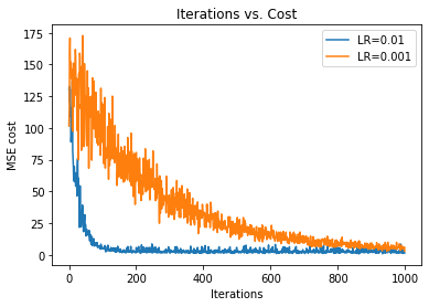
Next, we plot two graphs with different learning rates to see the effect of learning rate in optimization. In the following graph we can see that the graph with a higher learning rate (0.01) converges faster than the graph with a slower learning rate (0.001). As we learned in Part 1 of the Gradient Descent series, this is because the graph with the lower learning rate takes smaller steps.
17. Step — 17:
Let’s put it all together.
Number of Calculations:
Now, let’s count the number of calculations performed in the batch gradient descent algorithm.
Bias: (training examples) x (iterations) x (parameters) = 200 * 200 * 1 = 40000
Weights: (training examples) x (iterations) x (parameters) = 200 * 200 *3 = 120000
Stochastic Gradient Descent
In the batch gradient descent algorithm, we consider all the training examples for all the iterations of the algorithm. But, if our dataset has a large number of training examples and/or features, then it gets computationally expensive to calculate the parameter values. We know our machine learning algorithm will yield more accuracy if we provide it with more training examples. But, as the size of the dataset increases, the computations associated with it also increase. Let’s take an example to understand this in a better way.
Batch Gradient Descent (BGD)
Number of training examples per iterations = 1 million = 1⁰⁶
Number of iterations = 1000 = 1⁰³
Number of parameters to be trained = 10000 = 1⁰⁴
Total computations = 1⁰⁶*1⁰³*1⁰⁴=1⁰¹³
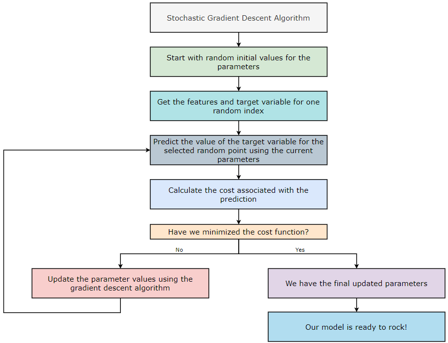
Now, if we look at the above number, it does not give us excellent vibes! So we can say that using the Batch Gradient Descent algorithm does not seem efficient. So, to deal with this problem, we use the Stochastic Gradient Descent (SGD) algorithm. The word “Stochastic” means random. So, instead of performing calculation on all the training examples of a dataset, we take one random example and perform the calculations on that. Sounds interesting, doesn’t it? We just consider one training example per iteration in the Stochastic Gradient Descent (SGD) algorithm. Let’s see how effective Stochastic Gradient Descent is based on its calculations.
Stochastic Gradient Descent (SGD):
Number of training examples per iterations = 1
Number of iterations = 1000 = 1⁰³
Number of parameters to be trained = 10000 = 1⁰⁴
Total computations = 1 * 1⁰³*1⁰⁴=1⁰⁷
Comparison with Batch Gradient Descent:
Total computations in BGD = 1⁰¹³
Total computations in SGD = 1⁰⁷
Evaluation: SGD is ¹⁰⁶ times faster than BGD in this example.
Note: Please be aware that our cost function might not necessarily go down as we just take one random training example every iteration, so don’t worry. However, the cost function will gradually decrease as we perform more and more iterations.
Now, let’s see how the Stochastic Gradient Descent (SGD) algorithm is implemented.
1. Step — 1:
First, we are downloading the data file from the GitHub repository.
2. Step — 2:
Next, we are importing some required libraries to read, manipulate, and visualize the data.
3. Step — 3:
Next, we are reading the data file, and then printing the first five rows of it.
4. Step — 4:
Next, we are dividing the dataset into features and target variables.
Dimensions: X = (200, 3) & Y = (200, )
5. Step — 5:
To perform matrix calculations in further steps, we need to reshape the target variable.
Dimensions: X = (200, 3) & Y = (200, 1)
6. Step — 6:
Next, we are normalizing the dataset.
Dimensions: X = (200, 3) & Y = (200, 1)
7. Step — 7:
Next, we are getting the initial values for the bias and weights matrices. We will use these values in the first iteration while performing forward propagation.
Dimensions: bias = (1, 1) & weights = (1, 3)
8. Step — 8:
Next, we perform the forward propagation step. This step is based on the following formula.
Dimensions: predicted_value = (1, 1)+(200, 3)*(3,1) = (1, 1)+(200, 1) = (200, 1)
9. Step — 9:
Next, we’ll calculate the cost associated to our prediction. The formula used for this step is as follows. Because there will only be one value of the error, we won’t need to divide the cost function by the size of the dataset or add up all the cost values.
Dimensions: cost = scalar value
10. Step — 10:
Next, we update the parameter values of weights and bias using the gradient descent algorithm. This step is based on the following formulas. Please note that the reason why we are not summing over the values of the weights is that our weight matrix is not a 1*1 matrix. Also, in this case, since we have only one training example, we won’t need to perform the summation over all the examples. The updated formula is given as follows.
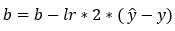
Dimensions: db = (1, 1)
Dimensions: dw = (1, 200) * (200, 3) = (1, 3)
Dimensions: bias = (1, 1) & weights = (1, 3)
11. Step — 11:
12. Step — 12:
Next, we are actually calling the function to get the final results. Please note that we are running the entire code for 200 iterations. Also, here we have specified the learning rate of 0.01.
13. Step — 13:
Next, we print the final weights values after all the iterations are done.
14. Step — 14:
Next, we print the final bias value after all the iterations are done.
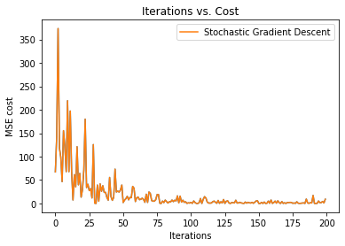
15. Step — 15:
Next, we are plotting the graph of iterations vs. cost.
16. Step — 16:
Next, we plot two graphs with different learning rates to see the effect of learning rate in optimization. In the following graph we can see that the graph with a higher learning rate (0.01) converges faster than the graph with a slower learning rate (0.001). Again, we know this because the graph with a lower learning rate takes smaller steps.
17. Step — 17:
Putting it all together.
Calculations:
Now, let’s count the number of calculations performed in implementing the batch gradient descent algorithm.
Bias: (training examples) x (iterations) x (parameters) = 1* 200 * 1 = 200
Weights: (training examples) x (iterations) x (parameters) = 1* 200 *3 = 600
Mini-Batch Gradient Descent Algorithm:
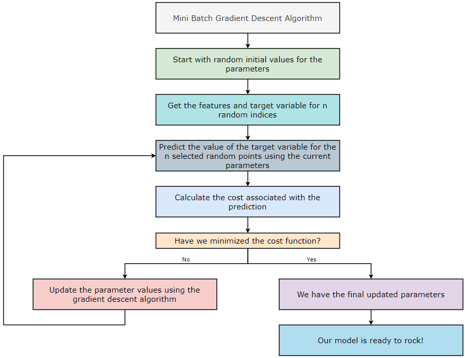
In the Batch Gradient Descent (BGD) algorithm, we consider all the training examples for all the iterations of the algorithm. However, in the Stochastic Gradient Descent (SGD) algorithm, we only consider one random training example. Now, in the Mini-Batch Gradient Descent (MBGD) algorithm, we consider a random subset of training examples in each iteration. Since this is not as random as SGD, we reach closer to the global minimum. However, MBGD is susceptible to getting stuck into local minima. Let’s take an example to understand this in a better way.
Batch Gradient Descent (BGD):
Number of training examples per iterations = 1 million = 1⁰⁶
Number of iterations = 1000 = 1⁰³
Number of parameters to be trained = 10000 = 1⁰⁴
Total computations = 1⁰⁶*1⁰³*1⁰⁴=1⁰¹³
Stochastic Gradient Descent (SGD):
Number of training examples per iterations = 1
Number of iterations = 1000 = 1⁰³
Number of parameters to be trained = 10000 = 1⁰⁴
Total computations = 1*1⁰³*1⁰⁴ = 1⁰⁷
Mini Batch Gradient Descent (MBGD):
Number of training examples per iterations = 100 = 1⁰²
→Here, we are considering 1⁰² training examples out of 1⁰⁶.
Number of iterations = 1000 = 1⁰³
Number of parameters to be trained = 10000 = 1⁰⁴
Total computations = 1⁰²*1⁰³*1⁰⁴=1⁰⁹
Comparison with Batch Gradient Descent (BGD):
Total computations in BGD = 1⁰¹³
Total computations in MBGD = 1⁰⁹
Evaluation: MBGD is 1⁰⁴ times faster than BGD in this example.
Comparison with Stochastic Gradient Descent (SGD):
Total computations in SGD = 1⁰⁷
Total computations in MBGD = 1⁰⁹
Evaluation: SGD is 1⁰² times faster than MBGD in this example.
Comparison of BGD, SGD, and MBGD:
Total computations in BGD= 1⁰¹³
Total computations in SGD= 1⁰⁷
Total computations in MBGD = 1⁰⁹
Evaluation: SGD > MBGD > BGD
Note: Please be aware that our cost function might not necessarily go down as we are taking a random sample of the training examples every iteration. However, the cost function will gradually decrease as we perform more and more iterations.
Now, let’s see how the Mini-Batch Gradient Descent (MBGD) algorithm is implemented in practice.
1. Step — 1:
First, we are downloading the data file from the GitHub repository.
2. Step — 2:
Next, we are importing some required libraries to read, manipulate, and visualize the data.
3. Step — 3:
Next, we are reading the data file, and then print the first five rows of it.
4. Step — 4:
Next, we are dividing the dataset into features and target variables.
Dimensions: X = (200, 3) & Y = (200, )
5. Step — 5:
To perform matrix calculations in further steps, we need to reshape the target variable.
Dimensions: X = (200, 3) & Y = (200, 1)
6. Step — 6:
Next, we are normalizing the dataset.
Dimensions: X = (200, 3) & Y = (200, 1)
7. Step — 7:
Next, we are getting the initial values for the bias and weights matrices. We will use these values in the first iteration while performing forward propagation.
Dimensions: bias = (1, 1) & weights = (1, 3)
8. Step — 8:
Next, we are performing the forward propagation step. This step is based on the following formula.
Dimensions: predicted_value = (1, 1)+(200, 3)*(3,1) = (1, 1)+(200, 1) = (200, 1)
9. Step — 9:
Next, we are going to calculate the cost associated with our prediction. This step is based on the following formula.
Dimensions: cost = scalar value
10. Step — 10:
Next, we update the parameter values of weights and bias using the gradient descent algorithm. This step is based on the following formulas. Please note that the reason why we are not summing over the values of the weights is that our weight matrix is not a 1*1 matrix.
Dimensions: db = sum(200, 1) = (1 , 1)
Dimensions: dw = (1, 200) * (200, 3) = (1, 3)
Dimensions: bias = (1, 1) & weights = (1, 3)
11. Step — 11:
Next, we are going to use all the functions we just defined to run the gradient descent algorithm. Also, we are creating an empty list called cost_list to store the cost values of all the iterations. We will use this list to plot a graph in further steps.
12. Step — 12:
Next, we are actually calling the function to get the final results. Please note that we are running the entire code for 200 iterations. Also, here we have specified the learning rate of 0.01.
13. Step — 13:
Next, we print the final weights values after all the iterations are done.
14. Step — 14:
Next, we print the final bias value after all the iterations are done.
15. Step — 15:
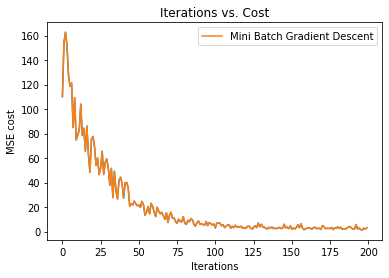
Next, we are plotting the graph of iterations vs. cost.
16. Step — 16:
Next, we plot two graphs with different learning rates to see the effect of learning rate in optimization. In the following graph we can see that the graph with a higher learning rate (0.01) converges faster than the graph with a slower learning rate (0.001). The reason behind it is that the graph with lower learning rate takes smaller steps.
17. Step — 17:
Putting it all together.
Calculations:
Now, let’s count the number of calculations performed in implementing the batch gradient descent algorithm.
Bias: (training examples) x (iterations) x (parameters) = 20 * 200 * 1 = 4000
Weights: (training examples) x (iterations) x (parameters) = 20 * 200 *3 = 12000
Graph comparisons:
End Notes:
And just like that, we’re at the end of the Gradient Descent series! In this installment, we went deep into the code to look at how three of the major types of gradient descent algorithms perform next to each other, summed up by these handy notes:
1. Batch Gradient Descent
Accuracy → High
Time → More
2. Stochastic Gradient Descent
Accuracy → Low
Time → Less
3. Mini-Batch Gradient Descent
Accuracy → Moderate
Time → Moderate
We hope you enjoyed this series and learned something new, no matter your starting point or machine learning background. Knowing this essential algorithm and its variants will likely prove valuable as you continue on your AI journey and understand more about both the technical and grand aspects of this incredible technology. Keep an eye out for other blogs offering, even more, machine learning lessons, and stay curious!

Resources:
- Batch Gradient Descent — Google Colab, GitHub
- Stochastic Gradient Descent — Google Colab, GitHub
- Mini Batch Gradient Descent — Google Colab, GitHub
Citation:
For attribution in academic contexts, please cite this work as:
Shukla, et al., “The Gradient Descent Algorithm & its Variants”, Towards AI, 2022
BibTex Citation:
@article{pratik_2022,
 title={The Gradient Descent Algorithm & its Variants},
 url={https://towardsai.net/neural-networks-with-python},
 journal={Towards AI},
 publisher={Towards AI Co.},
 author={Pratik, Shukla},
 editor={Lauren, Keegan},
 year={2022},
 month={Oct}
}
References:
The Gradient Descent Algorithm and its Variants was originally published in Towards AI on Medium, where people are continuing the conversation by highlighting and responding to this story.
Join thousands of data leaders on the AI newsletter. It’s free, we don’t spam, and we never share your email address. Keep up to date with the latest work in AI. From research to projects and ideas. If you are building an AI startup, an AI-related product, or a service, we invite you to consider becoming a sponsor.
Published via Towards AI
Towards AI Academy
We Build Enterprise-Grade AI. We'll Teach You to Master It Too.
15 engineers. 100,000+ students. Towards AI Academy teaches what actually survives production.
Start free — no commitment:
→ 6-Day Agentic AI Engineering Email Guide — one practical lesson per day
→ Agents Architecture Cheatsheet — 3 years of architecture decisions in 6 pages
Our courses:
→ AI Engineering Certification — 90+ lessons from project selection to deployed product. The most comprehensive practical LLM course out there.
→ Agent Engineering Course — Hands on with production agent architectures, memory, routing, and eval frameworks — built from real enterprise engagements.
→ AI for Work — Understand, evaluate, and apply AI for complex work tasks.
Note: Article content contains the views of the contributing authors and not Towards AI.
Related posts


Recent Posts


")