Mathematical Intuition behind the Gradient Descent Algorithm

Author(s): Towards AI Editorial Team

Originally published on Towards AI the World’s Leading AI and Technology News and Media Company. If you are building an AI-related product or service, we invite you to consider becoming an AI sponsor. At Towards AI, we help scale AI and technology startups. Let us help you unleash your technology to the masses.

Deriving Gradient Descent Algorithm for Mean Squared Error

Author(s): Pratik Shukla

“The mind is not a vessel to be filled, but a fire to be kindled.” — Plutarch

The Gradient Descent Series of Blogs:

1. The Gradient Descent Algorithm
2. Mathematical Intuition behind the Gradient Descent Algorithm (You are here!)
3. The Gradient Descent Algorithm & its Variants

Table of contents:

1. Introduction
2. Derivation of the Gradient Descent Algorithm for Mean Squared Error
3. Working Example of the Gradient Descent Algorithm
4. End Notes
5. References and Resources

Introduction:

Welcome! Today, we’re working on developing a strong mathematical intuition on how the Gradient Descent algorithm finds the best values for its parameters. Having this sense can help you catch mistakes in machine learning outputs and get even more comfortable with how the gradient descent algorithm makes machine learning so powerful. In the pages to follow, we will derive the equation of the gradient descent algorithm for the mean squared error function. We will use the results of this blog to code the gradient descent algorithm. Let’s dive into it!

Derivation of the Gradient Descent Algorithm for Mean Squared Error:

1. Step — 1:

The input data is shown in the matrix below. Here, we can observe that there are m training examples and n number of features.

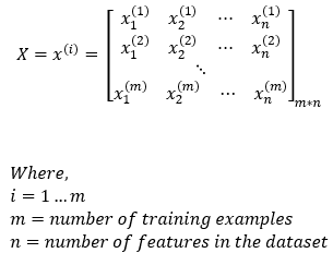
Dimensions: X = (m, n)

2. Step — 2:

The expected output matrix is shown below. Our expected output matrix will be of size m*1 because we have m training examples.

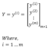
Dimensions: Y = (m, 1)

3. Step — 3:

We will add a bias element in our parameters to be trained.

Dimensions: α = (1, 1)

4. Step — 4:

In our parameters, we have our weight matrix. The weight matrix will have n elements. Here, n is the number of features of our training dataset.

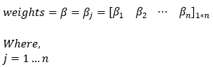
Dimensions: β = (1, n)

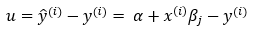
5. Step — 5:

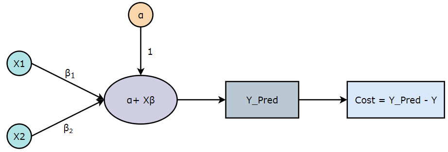
The predicted values for each training examples are given by,

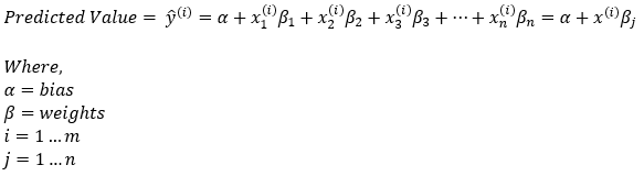
Please note that we are taking the transpose of the weights matrix (β) to make the dimensions compatible with matrix multiplication rules.

Dimensions: predicted_value = (1, 1) + (m, n) * (1, n)

— Taking the transpose of the weights matrix (β) —

Dimensions: predicted_value = (1, 1) + (m, n) * (n, 1) = (m, 1)

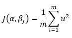
6. Step — 6:

The mean squared error is defined as follows.

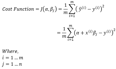
Dimensions: cost = scalar function

7. Step — 7:

We will use the following gradient descent rule to determine the best parameters in this case.

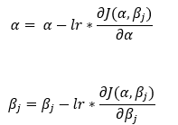
Dimensions: α = (1, 1) & β = (1, n)

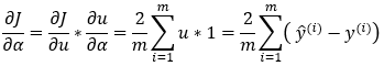
8. Step — 8:

Now, let’s find the partial derivative of the cost function with respect to the bias element (α).

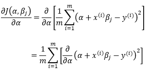
Dimensions: (1, 1)

9. Step — 9:

Now, we are trying to simplify the above equation to find the partial derivatives.

Dimensions: u = (m, 1)

10. Step — 10:

Based on Step — 9, we can write the cost function as,

Dimensions: scalar function

11. Step — 11:

Next, we will use the chain rule to calculate the partial derivative of the cost function with respect to the intercept (α).

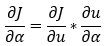
Dimensions: (m, 1)

12. Step — 12:

Next, we are calculating the first part of the partial derivative of Step — 11.

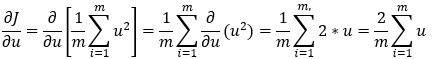
Dimensions: (m, 1)

13. Step — 13:

Next, we calculate the second part of the partial derivative of Step — 11.

Dimensions: scalar function

14. Step — 14:

Next, we multiply the results of Step — 12 and Step — 13 to find the final results.

Dimensions: (m, 1)

15. Step — 15:

Next, we will use the chain rule to calculate the partial derivative of the cost function with respect to the weights (β).

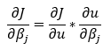
Dimensions: (1, n)

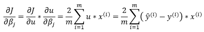
16. Step — 16:

Next, we calculate the second part of the partial derivative of Step — 15.

Dimensions: (m, n)

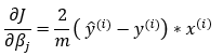
17. Step — 17:

Next, we multiply the results of Step — 12 and Step — 16 to find the final results of the partial derivative.

Now, since we want to have n values of weight, we will remove the summation part from the above equation.

Please note that here we will have to transpose the first part of the calculations to make it compatible with the matrix multiplication rules.

Dimensions: (m, 1) * (m, n)

— Taking the transpose of the error part —

Dimensions: (1, m) * (m, n) = (1, n)

18. Step — 18:

Next, we put all the calculated values in Step — 7 to calculate the gradient rule for updating α.

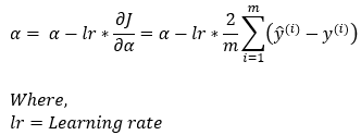
Dimensions: α = (1, 1)

19. Step — 19:

Next, we put all the calculated values in Step — 7 to calculate the gradient rule for updating β.

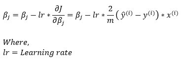
Please note that we must transpose the error value to make the function compatible with matrix multiplication rules.

Dimensions: β = (1, n) — (1, n) = (1, n)

Working Example of the Gradient Descent Algorithm:

Now, let’s take an example to see how the gradient descent algorithm finds the best parameter values.

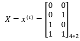
1. Step — 1:

The input data is shown in the matrix below. Here, we can observe that there are 4 training examples and 2 features.

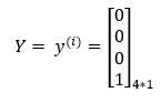
2. Step — 2:

The expected output matrix is shown below. Our expected output matrix will be of size 4*1 because we have 4 training examples.

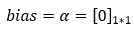
3. Step — 3:

We will add a bias element in our parameters to be trained. Here, we are choosing the initial value of 0 for bias.

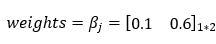
4. Step — 4:

In our parameters, we have our weight matrix. The weight matrix will have 2 elements. Here, 2 is the number of features of our training dataset. Initially, we can choose any random numbers for the weights matrix.

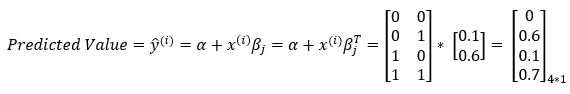
5. Step — 5:

Next, we are going to predict the values using our input matrix, weight matrix, and bias.

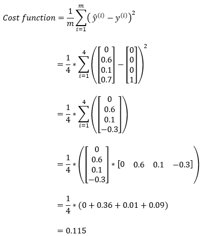
6. Step — 6:

Next, we calculate the cost using the following equation.

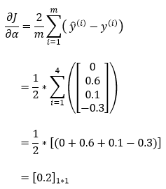
7. Step — 7:

Next, we are calculating the partial derivative of the cost function with respect to the bias element. We’ll use this result in the gradient descent algorithm to update the value of the bias parameter.

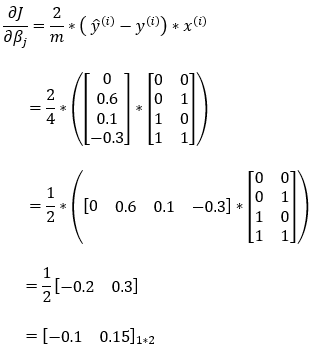
8. Step — 8:

Next, we are calculating the partial derivative of the cost function with respect to the weights matrix. We’ll use this result in the gradient descent algorithm to update the value of the weights matrix.

9. Step — 9:

Next, we are defining the value of the learning rate. Learning rate is the parameter which controls the speed of how fast our model learns.

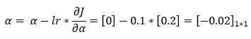
10. Step — 10:

Next, we are using the gradient descent rule to update the parameter value of the bias element.

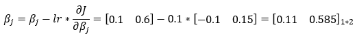
11. Step — 11:

Next, we are using the gradient descent rule to update the parameter values of the weights matrix.

12. Step — 12:

Now, we repeat this process for a number of iterations to find the best parameters for our model. In each iteration, we use the updated values of our parameters.

End Notes:

So, this is how we find the updated rules using the gradient descent algorithm for the mean squared error. We hope this sparked your curiosity and made you hungry for more machine learning knowledge. We will use the rules we derived here to implement the gradient descent algorithm in future blogs, so don’t miss the third installment in the Gradient Descent series where it all comes together — the grand finale!

Citation:

For attribution in academic contexts, please cite this work as:

Shukla, et al., “Mathematical Intuition behind the Gradient Descent Algorithm”, Towards AI, 2022

BibTex Citation:

@article{pratik_2022, 
 title={Mathematical Intuition behind the Gradient Descent Algorithm}, 
 url={https://towardsai.net/neural-networks-with-python}, 
 journal={Towards AI}, 
 publisher={Towards AI Co.}, 
 author={Pratik, Shukla},
 editor={Lauren, Keegan},  
 year={2022}, 
 month={Oct}
}

References and Resources:

1. Gradient descent — Wikipedia

---

Mathematical Intuition behind the Gradient Descent Algorithm was originally published in Towards AI on Medium, where people are continuing the conversation by highlighting and responding to this story.

Join thousands of data leaders on the AI newsletter. It’s free, we don’t spam, and we never share your email address. Keep up to date with the latest work in AI. From research to projects and ideas. If you are building an AI startup, an AI-related product, or a service, we invite you to consider becoming a sponsor.

Published via Towards AI