Exploration of CDFs: Their Applications in Data Science

Author(s): Ghadah AlHabib

Originally published on Towards AI.

Introduction to CDFs

Cumulative Distribution Functions (CDF) are functions that represent the probability of a random variable X that takes on a value less than or equal to a specific value x. It’s the cumulative probability associated with a distribution.

Use Case of using CDFs: Analyzing Customer Wait Times to Optimize Service Efficiency

The use of CDFs in this example is to understand the overall wait time experience of customers. It allows business owners to specify certain thresholds like the 80th percentile and set measurable goals based on the distribution of their data. For instance, if a business aims to increase customer satisfaction by reducing wait times, the CDF can help in providing a clear target and pinpoint specific wait times to aim for. So, “We want X% of our customers to be served within Y minutes”.

Let’s dive into the code:

Step 1: Dataset

First, we will generate a synthetic dataset to simulate realistic data attributes. CustomerID gives each observation a unique identifier, and timestamps give a specific time point to each observation.

import numpy as np
import pandas as pd
import matplotlib.pyplot as plt

# Seed for reproducibility
np.random.seed(42)

# Generate positive wait times using an absolute value of a normal distribution
wait_times = np.abs(np.random.normal(8, 3, 1000))
customer_ids = range(1, 1001)
timestamps = pd.date_range(start='2024-01-01 08:00', periods=1000, freq='T') # One-minute intervals

df = pd.DataFrame({
 'CustomerID': customer_ids,
 'Timestamp': timestamps,
 'WaitTime': wait_times
})

Why did we use a normal distribution to simulate the generation? Primarily for simplicity and illustrative purposes. We could use other distributions such as the exponential distribution. So, depending on your data, whether it’s skewed or bounded, you’ll be able to choose the most suitable distribution.

Step 2: Construct the CDF

sorted_df = df.sort_values('WaitTime').reset_index(drop=True)
sorted_df['CDF'] = (sorted_df.index + 1) / len(sorted_df)

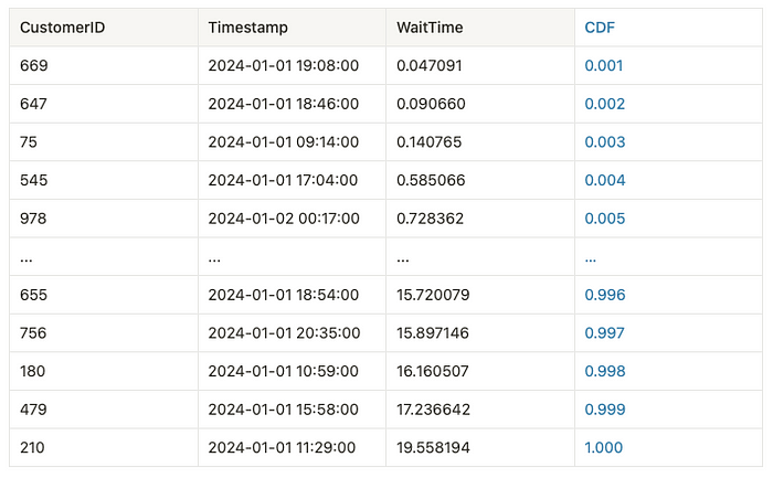
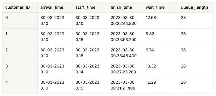
The values are sorted by the wait time to calculate the cumulative sum of probabilities up to a certain wait time. Then, the CDF for each wait time is calculated by taking the index (which, after sorting, represents the number of values less than or equal to the current wait time) and dividing it by the total number of observations (rows). This computes the proportion of customers who have waited for less than or equal to each specific wait time.

Below we can see the sorted wait time along with the CDF value:

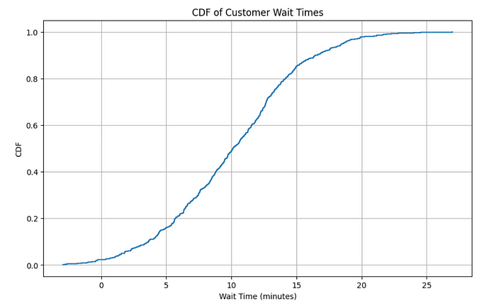
Step 3: Let’s plot the CDF

plt.figure(figsize=(10, 6))
plt.step(sorted_df['WaitTime'], sorted_df['CDF'], where='post')
plt.xlabel('Wait Time (minutes)')
plt.ylabel('CDF')
plt.title('CDF of Customer Wait Times')
plt.grid(True)
plt.show()

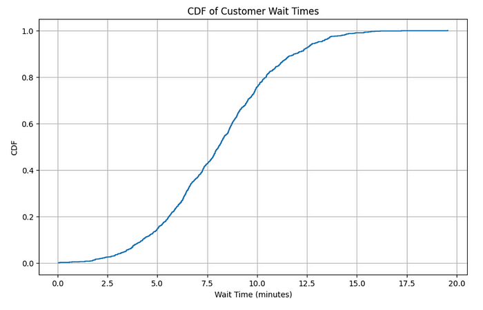
Step 4: Let’s extract insights! What kind of questions does this graph answer?

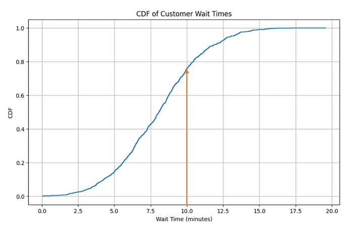
Question 1: What percentage of customers experience a wait time of less than 10 minutes?

wait_time_threshold = 10
sorted_df[sorted_df['WaitTime'] < wait_time_threshold]['CDF'].max() * 100

# Output: 75.70% of customers wait less than 10 minutes.

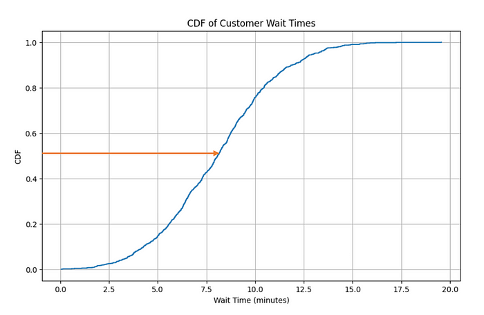
Question 2: How long do 50% of the customers wait?

percentage = 0.50
sorted_df[sorted_df['CDF'] <= percentage]['WaitTime'].max()

# Output: 50% of the customers wait less than or equal to 8.07 minutes.

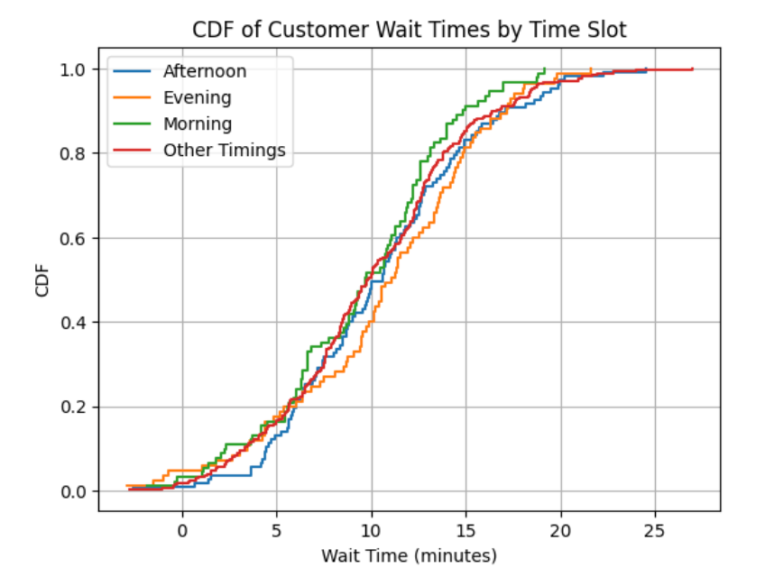
Question 3: Give me more insights about resource allocation. Does the timing of the day affect the wait time distribution?

• If the CDF varies significantly at different times: need for differential resource allocation to improve customer wait times during peak hours. Longer waiting times; peak hours.
• If the CDF remains stable and no dramatic difference in customer wait times: balanced resource allocation.

Let’s explore the implementation:

sorted_df['Hour'] = sorted_df['Timestamp'].dt.hour

def assign_time_slot(hour):
 if 8 <= hour < 12:
 return 'Morning'
 elif 12 <= hour < 16:
 return 'Afternoon'
 elif 16 <= hour < 20:
 return 'Evening'
 else:
 return 'Other Timings'

sorted_df['TimeSlot'] = sorted_df['Hour'].apply(assign_time_slot)

grouped = sorted_df.groupby('TimeSlot')

for name, group in grouped:
 sorted_group = group.sort_values('WaitTime').reset_index(drop=True)
 sorted_group['CDF'] = (sorted_group.index + 1) / len(sorted_group)
 plt.step(sorted_group['WaitTime'], sorted_group['CDF'], where='post', label=name)

plt.xlabel('Wait Time (minutes)')
plt.ylabel('CDF')
plt.title('CDF of Customer Wait Times by Time Slot')
plt.legend()
plt.grid(True)
plt.show()

Interpreting the results:

The curves for each time slot are close to each other, indicating that the distribution of wait times does not change significantly throughout the day and there is no significant peak time. Therefore, it’s a good indicator that resource allocation is balanced and that there’s a consistent service experience throughout the day.

Let’s use a real dataset from Kaggle!

Join thousands of data leaders on the AI newsletter. Join over 80,000 subscribers and keep up to date with the latest developments in AI. From research to projects and ideas. If you are building an AI startup, an AI-related product, or a service, we invite you to consider becoming a sponsor.

Published via Towards AI