The Architecture of Mistral’s Sparse Mixture of Experts (S〽️⭕E)

Author(s): JAIGANESAN

Originally published on Towards AI.

Exploring Feed Forward Networks, Gating Mechanism, Mixture of Experts (MoE), and Sparse Mixture of Experts (SMoE).

Introduction:🥳

In this article, we’ll dive deeper into the specifics of Mistral’s SMoE (Sparse Mixture of Experts)[2] architecture. If you’re new to this topic or need a refresher, I recommend checking out my previous articles, “LLM: In and Out” and “Breaking Down Mistral 7B”, which cover the basics of LLMs and the Mistral 7B architecture.

Large Language Model (LLM)🤖: In and Out

Delving into the Architecture of LLM: Unraveling the Mechanics Behind Large Language Models like GPT, LLAMA, etc.

pub.towardsai.net

Breaking down Mistral 7B ⚡🍨

Exploring Mistral’s Rotary positional Embedding, Sliding Window Attention, KV Cache with rolling buffer, and…

pub.towardsai.net

If you’re already familiar with the inner workings of Mistral 7B[1], then you can continue this article.

Before we explore the topic further, we first need to understand Mistral’s 8 X 7B (MoE) Architecture. According to the research paper, the main distinction between Mistral 7B and Mistral 8 X 7B (SMoE) lies in adding the Mixture of Experts layer in the Mistral 8 X 7B (SMoE).

Let’s look closer at the Mistral 8 x 7B architecture. This architecture has a model dimension of 4096. It’s made up of 32 layers. The model uses 32 heads and 8 key value (KV) heads. Each head in the model has a dimension of 128. The feed-forward network (FFN) has a hidden dimension of 14336. The context length is 32768 and the vocabulary size is 32000 😯 And the Number of Experts in the MoE layer is 8 and the Top 2 Experts are selected for each token.

If you have any doubt, about where this architecture comes from, I recommend you to check out the Mistral inference Github code and Research paper.

GitHub – mistralai/mistral-inference: Official inference library for Mistral models

Official inference library for Mistral models. Contribute to mistralai/mistral-inference development by creating an…

github.com

In this article, we’ll explore three key concepts that make Mistral’s MoE architecture ✅.

Here’s what I am going to explore: 🛤

✨ Feed Forward Network (FFN)

✨ Mixture of Experts (MoE)

✨ Mistral’s Sparse Mixture of Experts (SMoE)

1. Feed Forward Network (SwiGLU FFN)

Note: If you’ve already read my previous article on Mistral 7B, feel free to skip this section and jump straight to the Mixture of Experts part.

Before we dive into the Mixture of Experts (MoE), We should Understand the Experts. Yes, What you read is right, Experts in MoE are nothing but a Feed-forward Network. So Let’s dive into the Feed-Forward Network (FFN) of the Mistral.

Image 2: Numbers in the images are input and output dimensions from respective neurons and input layer.

If you have a question why do we need FFN?

The answer is that attention gives the relationship between words (Semantic, syntactic relationships, and how one words are related to others). But FFN learns to represent the words, It actually learns to write the sequence of the words from the attention information. It learns to write the next word using the context (Auto regressive property).

The FFN (Neural Network) is backed by the Universal approximation theorem (UAT). What does UAT say? It can approximate any ideal function in the real world. It is the same thing that the FFN learns to represent the language and to write the words from the attention information.

The FFN takes the input from the attention layer, which has undergone RMS normalization, as its input.

For Example, Let’s take the input token size as 9. It has gone through the Attention layer and Normalization layer. This FFN input matrix has a shape of (9, 4096), where 9 represents the number of tokens or sequence length (i.e., the number of vectors), and 4096 is the model dimension.

Before we dive into the illustration of a feed-forward network, let’s take a closer look at the code of a FeedForward Network from Mistral 8 x 7B.

class FeedForward(nn.Module):
 def __init__(self, args: ModelArgs):
 super().__init__()
 # Image 3 will represents pytorch linear layer operation.
 self.w1 = nn.Linear(args.dim, args.hidden_dim, bias=False)
 self.w2 = nn.Linear(args.hidden_dim, args.dim, bias=False)
 self.w3 = nn.Linear(args.dim, args.hidden_dim, bias=False)

 def forward(self, x) -> torch.Tensor:
 return self.w2(nn.functional.silu(self.w1(x)) * self.w3(x))

# SwiGLU = nn.functional.silu(self.w1(x)) * self.w3(x) 
# self.w3(x) = Acts as Gating Mechanism 
# Swish Activation(Beta=1) = nn.functional.silu(self.w1(x))
# By doing this we Introduce Non-linearity in element wise and Preserve the high magnitude of the vector.

Image 3: x is the input vector, A is the weight matrix, and b is the bias vector.

This code shows that there are two hidden layer operations, not two hidden layers fully connected. (SwiGLU Mechanism)

Let’s break it down: the input matrix is fed into two hidden layers, self.w1, and self.w3, and then multiplied point-wise. The self.w1 hidden layer goes SiLU activation, But self.w3 does not.

As we Know The Mistral Uses the SwiGLU activation Function (That has two hidden layer operations as you can understand from the code)

SwiGLU (x) = SiLU(W_1.x).(W_3.x)

Why do they use two hidden layer operations (SwiGLU)? From my understanding, they have used another hidden layer operation to maintain the Magnitude of the vector, Because SiLU will reduce the Magnitude of all vectors. When sigmoid output is multiplied by the input vector (x) their magnitude will decrease unless the sigmoid output is 1. So that’s why Mistral uses another hidden layer in FFN and multiplies the output with a SiLU-activated hidden layer to maintain the magnitude of the vector as high that will be given to the next layer or linear layer. Otherwise, it will lead to a Vanishing gradient problem. This Operation is called SwiGLU activation. It gives non-linearity to Each element and preserves the high magnitude.

There are two hidden layers’ weight matrices size of (14336,4096) as shown in images 4 and 4A.

Note: The Numbers in the Images are for illustration purposes only.

The Input vector is Multiplied with two hidden layer weight matrices separately and multiplied point-wise as shown in images 4 and 4A.

The FFN hidden layer resulting matrix, with a shape of (9,14336), is then fed into the FFN output layer and multiplied by the output layer Transposed weight matrix W_2, which has a shape of (14336, 4096). This results in a feed-forward layer output with a size of (9,4096) as shown in image 5.

Image 6 (Vanilla transformer FFN operation from Attention is all you need paper) provides a representation of the operations taking place within the Feed-Forward Network (FFN), which were previously explained in Images 4, and 4A ( x is the input vector, W1, W2, and W3 are weight matrix or parameters, Mistral didn’t use bias vector).

This decoder Layer 1 output is then fed into the next layer or linear layer if there is no next layer. This helps us to predict the next token. Mistral’s FFN operation is a little bit different as shown in the code above. I Want to give proof of how the FFN works, that is why I have given image 6.

2. Mixture of Experts (MoE)

To Understand the concept of the Sparse Mixture of Experts, it’s essential to first understand what the Mixture of Experts is. So, let’s explore the Mixture of Experts😊.

The Mixture of Experts is an ensemble method that brings together multiple expert models, similar to the Random Forest algorithm. Just as Random Forest is a collection of decision tree algorithms, the Mixture of Experts is a collection or ensemble of feedforward neural networks(FFN).

MoE’s Experts can handle different parts of the task or Input data. Each expert in the MoE is specialized to handle a specific part of the input data or a particular part of the problem. It helps each model to learn and perform well on its specialized tasks and gives better overall performance.

In complex tasks, different parts of the input data may have different characteristics. By using specialized Expert models that can handle these different characteristics, we can enhance the efficiency and accuracy of the system.

For Example, one expert might excel at generating good code, while another expert might be proficient in solving complex reasoning tasks, and another might be specialized at understanding grammar and producing good content.

By focusing on specific tasks or subsets of data, these experts can achieve higher accuracy compared to general models (Mistral 7B). Moreover, MoE can handle different modalities, like text, images, audio, and video.

Take a look at Image 7. You can see that an input, labeled as x, is being fed into all five experts in the Mixture of Experts (MoE) layer. Now, imagine a Gating Network, which is a linear layer that projects the input to produce logit scores for each token. These Logit scores are fed into the softmax function. All logit scores are converted into probability scores.

In the Mixture of Experts method, the input is fed into all the experts, and each expert generates an output. But here’s the key part: a score is assigned to each expert’s output, which determines how important that output is. This score doesn’t decide which expert to use; instead, it weighs the importance of each expert’s output.

The weight probabilities are represented as g1, g2, g3, g4, and g5 which are multiplied by the output of each expert. The result is a weighted sum of the token/vector, which is a combination of the outputs from all the experts.

Image 8 provides a clear illustration of the Gating Network in the Mixture of Experts’ working mechanism. Let’s break it down step by step. The output from the attention layer is passed through the Gating network.

The Gating Network plays a crucial role in the Mixture of Experts method. Gating Network learns which expert is best suited to handle each specific token, and it does this by assigning a weight to each expert for every token. simply, the Gating Network figures out which expert will represent each token in the most effective way possible.

This output, which has a size of (9,4096), is multiplied by the transposed weight matrix of the Gate network’s linear layer. The result is the Gating network output logits, which have a size of (9,5). Note that the number of experts is equal to the number of logits in each row (5 experts). This logit score gives the importance of experts with respect to the token.

Next, these output logits are converted into probabilities using the softmax function. This means that each row of logits is transformed into probabilities, and the sum of these probabilities equals 1.

To make it easier to understand, let’s take a single row or token from the attention layer output and use it as input for the Mixture of Experts (MoE). This input vector is fed into all the experts, which are nothing but feed-forward networks (FFNs) that we’ve seen before.

In this case, the input vector is represented as x_1, x_2, x_3, x_4, and x_5,(For each expert) and all the experts process this input vector. The result from all experts is five output vectors, each with a size of (1,4096).

To summarize, we have one input vector, but we get five output vectors. The input vector goes through all the experts in the MoE layer, and the experts learn to represent the token in different ways.

Now, let’s take the five output vectors from the experts and multiply them with the probability scores generated by the Gating network. As we saw in Image 8, the Gating network gives a probability score for each token with respect to each of the five experts.

These probability scores are then multiplied with the corresponding output vectors from the experts. Finally, all these vectors are summed up to produce a single vector with a size of (1,4096). This is how the weighted sum operation works in the Mixture of Experts layer as shown in image 10.

The output from the Mixture of Experts layer is then passed on to the next decoder layer or the output linear layer.

As we continue to train the experts, Each expert starts to specialize in different tasks or different parts of the training data, becoming more proficient in handling specific types of tokens or inputs. But that’s not all — each expert also develops some knowledge about the specializations of the other experts.

This means that even though each expert has its own area of expertise, they’re not isolated from one another. actually, they work together. This enables the model to handle a wide range of tasks and inputs with good accuracy and efficiency.

While the Mixture of Experts architecture has its advantages, it’s not without its drawbacks 😞. As I mentioned earlier, continued training can lead to each expert specializing in its task, but this comes with its own set of challenges.

One of the main issues is that MoE involves a complex mechanism of combining and coordinating the learning of multiple experts along with the gating network. Each expert learns effectively and contributes appropriately can be a difficult task.

Additionally, there’s a risk of overfitting, which means the model may not generalize well.

The biggest problem with MoE is its computational expense. During both training and inference, each token is sent to all the experts, which means all experts are active for all tokens. This can be very costly in terms of computational resources. And during inference, the time it takes to process the input can increase significantly (Bottleneck in GPU operation and Saving), because all experts are active for all tokens.

3. Mistral’s Sparse Mixture of Experts (SMoE)

To address the disadvantages of the Mixture of Experts architecture, a new approach called Sparse Mixture of Experts was introduced by the researchers[3]. This approach is designed to reduce the computational cost and complexity of MoE.

In a Sparse MoE, each token is only sent to the top k experts, rather than all the experts in the MoE layer. This means that only a selected few experts are activated for each token, rather than all of the experts.

In the Mistral model, the router is responsible for selecting the top 2 experts for each token. This approach reduces the computational cost and makes the model more efficient, while still allowing the experts to specialize and learn effectively.

Image 12 (Sparse Mixture of Experts Equation): input tokens or vectors, represented by “x”. Multiple experts then process these inputs, defined as “E_i”. The gate, or router, plays an important role in selecting the top 2 experts that are best suited to handle the input/token. This selection is represented by “G(x)_i”. The number of experts is represented by “n”.

# Code from Mistral's MoE Inference
class MoeLayer(nn.Module):
 ...

 def forward:
 gate_logits = self.gate(inputs_squashed)
 weights, selected_experts = torch.topk(gate_logits, 
 self.args.num_experts_per_tok)

 weights = nn.functional.softmax(weights,dim=1,dtype=torch.float,
 ).type_as(inputs) # Selected weights get's into softmax function


class TransformerBlock(nn.Module):
 ...
 def forward:
 self.feed_forward = MoeLayer(
 experts=[FeedForward(args=args) for _ in range(args.moe.num_experts)],
 gate=nn.Linear(args.dim, args.moe.num_experts, bias=False),moe_args=args.moe,)

From this code, we can understand the gate (router) and how the top 2 experts are selected. To make it easier to visualize, I’ll explain the working mechanism using the images below.

As shown in Image 13, we have an input vector x fed into the Gating Network. The router or gate, uses a gating weight matrix represented by W_g to process the input. This operation is further explained in Image 14, which visually represents how the router handles the input vector/token.

As illustrated in Image 14, the attention layer produces an output with a size of (9,4096). This output is then multiplied by the transposed gating network weight matrix, which has a size of (4096, 8). The resulting matrix, known as the logits matrix, has a size of (9,8).

This logit matrix plays a crucial role in determining the top 2 experts for each input token. For example, considering the first token, the logits matrix suggests that experts 2 and 7 are the most suitable for processing this token.

The next step in the process is to apply the softmax function to the selected top 2 logits. This transforms the logits into probability scores, which are then used to calculate the weighted sum vector for each token.

The resulting probability scores provide a measure of how likely each of the top 2 experts is to produce the best output for a given token, allowing the model to combine their outputs to get both experts' representation of the token.

As shown in Image 15, the first token is fed into the selected top 2 experts (Experts 2 and 7)in the Sparse Mixture of Experts (SMoE) layer. Each expert is nothing but a Feed-Forward Network (FFN) layer, which we’ve seen earlier. The output of this process is two output vectors, each with a size of (1,4096), one from Expert 2 and one from Expert 7.

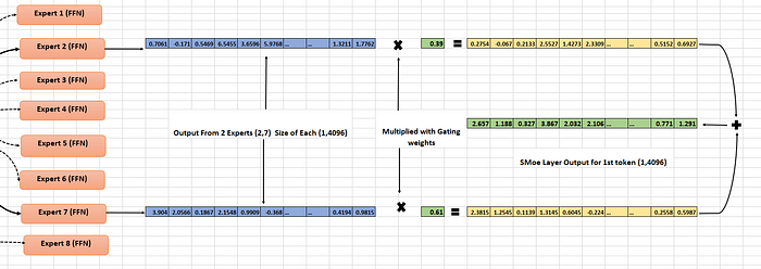
The next step is multiplying the experts' two output vectors with their corresponding softmax probability score, also known as gating weights. These weighted vectors are added together, resulting in a weighted sum vector for each token. This weighted sum vector is then fed into the next decoder layer or linear layer, which helps us predict the next token in the sequence.

One of its key benefits is that SMoE reduces the computational load. Here’s how: for each token, only two experts are activated,o as we know, which helps avoid bottlenecks or tradeoffs in GPUs. This, in turn, enables faster inference. Additionally, the SMoE method minimizes the risk of overfitting, allowing the model to learn more diversely and effectively.

In conclusion, we’ve explored the inner workings of Feed Forward Networks, Mixture of Experts, and Sparse Mixture of Experts. I hope this article has provided you with a clear understanding of these complex concepts. Stay tuned for the upcoming article, where we’ll delve into the variations of Mixture of Experts and Sparse Mixture of Experts, and uncover even more exciting insights into the world of AI.

Thanks for reading this article 🤩. If you found my article useful 👍, give it a👏😉! Feel free to follow for more insights.

Let’s also stay in touch on www.linkedin.com/in/jaiganesan-n/ 🌏❤️to keep the conversation going!

References :

[1] Albert Q. Jiang, Alexandre Sablayrolles, Arthur Mensch, Chris Bamford, Devendra Singh Chaplot. Mistral 7B (2023). Research paper (Arxiv).

[2] Albert Q. Jiang, Alexandre Sablayrolles, Antoine Roux, Arthur Mensch, Blanche Savary, Chris Bamford, Devendra Singh Chaplot. Mixtral of Experts (2024). Research paper (Arxiv).

[3] William Fedus, Jeff Dean, Barret Zoph. A Review of Sparse Expert models in deep learning (2022). Research paper (Arxiv).

[4] Ashish Vaswani, Noam Shazeer, Niki Parmar, Jakob Uszkoreit, Llion Jones, Attention is all you Need (2017). Research Paper (Arxiv)

Join thousands of data leaders on the AI newsletter. Join over 80,000 subscribers and keep up to date with the latest developments in AI. From research to projects and ideas. If you are building an AI startup, an AI-related product, or a service, we invite you to consider becoming a sponsor.

Published via Towards AI