


Introduction to Deep Learning with TensorFlow
Last Updated on January 7, 2023 by Editorial Team
Last Updated on August 26, 2020 by Editorial Team
Author(s): Satsawat Natakarnkitkul
Artificial Intelligence, Deep Learning
Gentle introduction and implementation of the top three types of ANNs; feed-forward neural networks, RNNs, and CNNs using TensorFlow
With the current advancement in data analytic and data science, many organization starts to implement a solution based on artificial neural networks (ANN) to automatically predict the outcome of the various business problem.
There are various types of ANN, for example; feed-forward neural network (artificial neuron), recurrent neural network (RNN), convolutional neural network (CNN), etc. In this article, we will go through all these three types of ANN. I have used the TensorFlow version 2.3.0 for all the examples shown here. Some commands and methods may be not available for the previous version.
Feed-Forward Neural Network
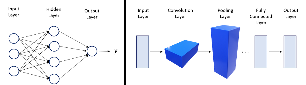
This is one of the simplest forms of ANN, where the input travels only in one direction. The data are passing through the input layer and exiting on the output layer. It may have hidden layers or not. As the name suggested, it only has front propagated and not backpropagation.
Tensorflow implementation can be done from the snippet code below, by using sequential of dense layer.
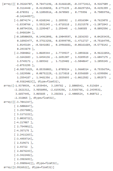
We can get the weight and bias of the neuron by calling model.get_weights(). The first one is the weights for 5 features input toward 16 neurons in the layer and the second array represents the bias of each 16 neurons. The third and fourth array represents the weight of output coming from the previous layer (16 neurons) and the bias of the output neuron.
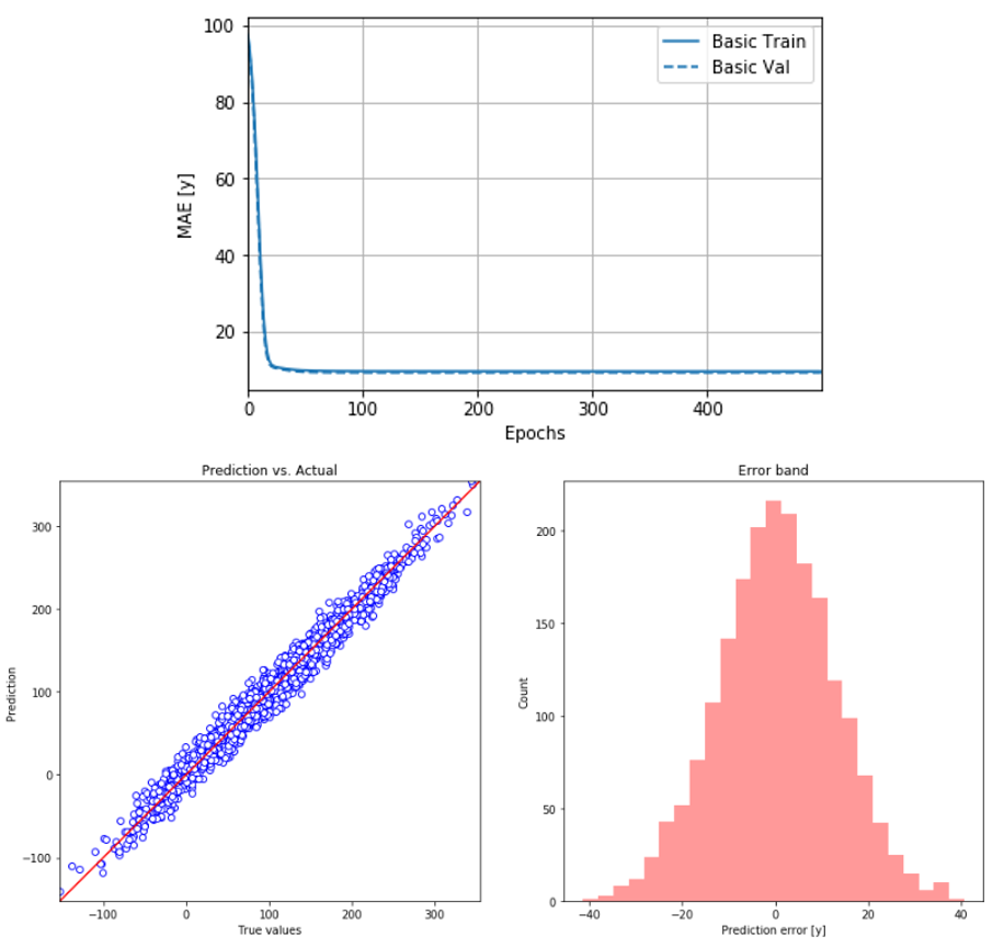
In addition, we can learn more about the model learning process (history) and model performance by visualizing the training log and prediction error.
Recurrent Neural Network, RNN
Recurrent neural networks are different from traditional feed-forward neural networks. Recurrent neural networks are designed to better handle sequential information. They introduce state variables to store past information, combine with the current inputs to determine the current outputs. Some common examples of RNN are based on text data and time-series data.
Let us visualize the RNN with a hidden state.
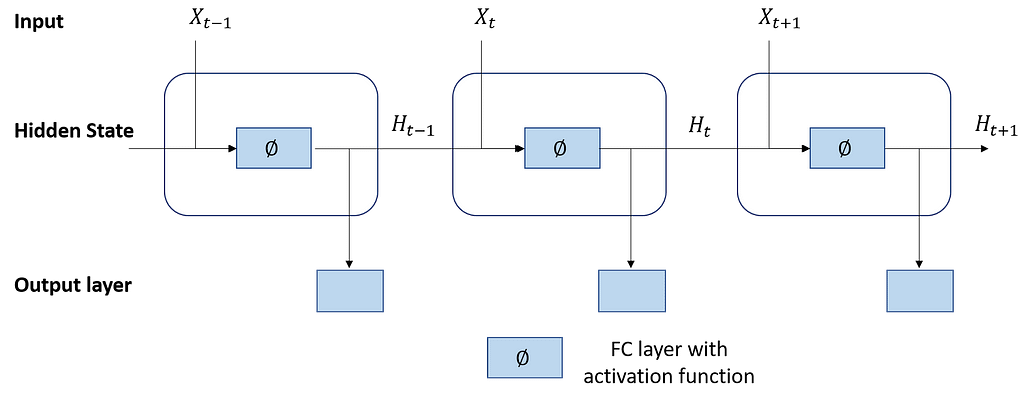
We can see that the calculation of the hidden variable of the current time step is determined by the input of the current time step together with the hidden variable of the previous time step. These activations are stored in the internal states of the network which can hold long-term temporal contextual information. This contextual information used to transform an input sequence into an output sequence. Hence, context is key for a recurrent neural network.
However, the RNN is not sufficient to solve today’s sequence learning problems, for example; numerical instability during gradient calculation.
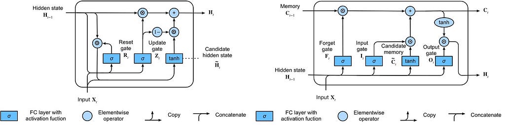
As mentioned, the networks have an internal state (storage) that can represent context information. The storage can also be replaced by another network or graph. Such controlled states refer to gated state or gated memory and are part of long short-term memory networks (LSTMs) and gated recurrent units (GRUs). The networks can also be called Feedback Neural Network.
RNNs can be one-directional and bidirectional. If we believe that there is a context around the data, not only just the data come before it. We should use bidirectional RNNs, for example, text data where the context comes in both before and after the word. For more explanation on RNN, I would suggest viewing this video.
Both GRUs and LSTMs consume the input shape of [batch size, time steps, features].
- Batch size is the number of samples for neural networks to see before adjusting the weights. The small batch size will reduce the speed of training but if the batch size is too big, the model will not be able to generalize and consume more memory (to keep the number of samples for each batch)
- Time steps are the units back in time for the neural network to see (i.e. time step = 30 can mean we look back and feed 30-day of data as input for one observation
- Features are the number of attributes used in each time step. Example if we use only stock’s closing price with 60 days time steps, feature size will only be 1
Below is the example of the implementation of both GRUs and LSTMs to predict Google’s stock price.
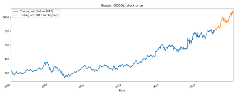
In general, when we use the recurrent neural network to predict the numeric value, we need to standardize the input values.
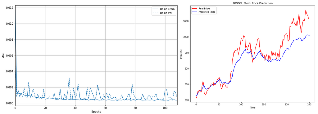
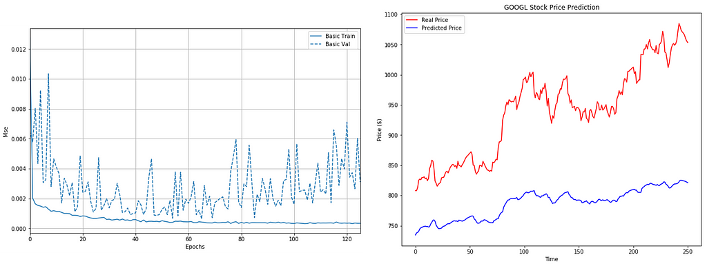
As we can see LSTM can detect the trend but there’re large rooms for improvement which can be made. However, in this post, I will focus on usage only.
In summary, GRUs are;
- Better at capturing dependencies for time series with large time step distances
- The reset gates help capture short-term dependencies while the update gates help capture long-term dependencies in time-series data
LSTMs have;
- Three types of gates (input, forget, and output gates) to control the flow of information
- The hidden layer output of LSTM includes hidden states and memory cells. The hidden states are passed into the output layer but the memory cells are entirely internal
- It can cope with vanishing and exploding gradients
Convolutional Neural Network, CNN
CNNs, like neural networks, are made up of neurons with learnable weights and biases. However, they are a powerful family of neural networks that are designed for computer vision. The application of CNNs related to image recognition, object detection, semantic segmentation, etc.
CNNs tend to be computationally efficient, both because they require fewer parameters than fully-connected architectures and because they are easy to parallelize across GPU. With these, CNNs have been used in a one-dimensional sequence structure (i.e. audio, text, and time-series data). Moreover, some have adapted the CNNs on graph-structured data and in the recommendation system. I would recommend reading the details of each function of convolutional, pooling layers in more detail here.
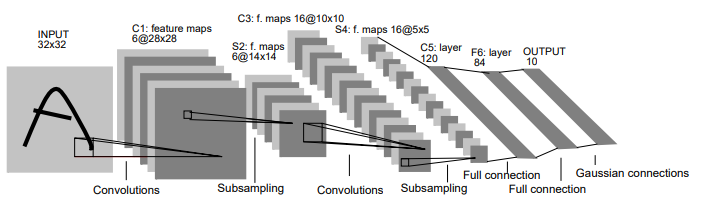
Typically for computer vision tasks, CNN takes the input of shape (image height, image width, color channels), ignoring the batch size. The color channels, or depth, refer to (R, G, B) color scheme.

Below is how we can implement a basic CNN model for classifying the images.
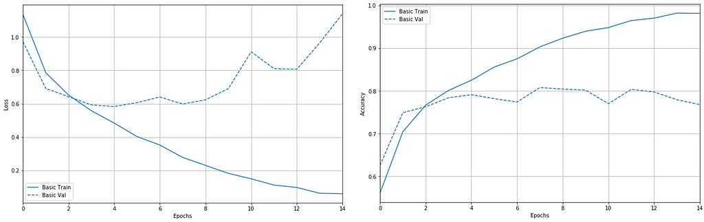
We can see that the model becomes over-fitting with training data and the performance is becoming worst on the validation data. The model performance on training data is 93.1% vs. testing data of 76.4%.
However, we can improve the model result by adding a data augmentation process to expand the training dataset, which helps the model to generalize better.
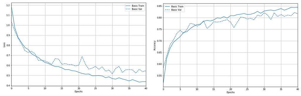
With this simple technique, the model is more generalized to the data. The accuracy towards training data is reduced to 85.1% but the testing accuracy is now at 81.7%.
In summary;
- Convolutional layers extract the feature from the input data
- Convolutional layers are arranged so that they gradually decrease the spatial resolution of the representations while increasing the number of channels
- It generally consists of convolutions, non-linearities, and often pooling operations
- At the end of the network, it connected to one or more fully-connected layers prior to computing the output
Endnote
I have introduced the most frequently used network types and their implementations using python and TensorFlow. For the full code used in this article, please refer to the GitHub repository or click here to read the notebook.
Once you fully understand each of these network types, you can combine them to solve more complicated problems, for example; parallel LSTMs to solve streaming data in real-time prediction, Convolutional LSTM to solve video problems (think as it is a sequence of images). Please refer to my GitHub repository below for the code and data.
Additional Reading and Github repository
- CS231n Convolutional Neural Networks for Visual Recognition
- 8. Recurrent Neural Networks – Dive into Deep Learning 0.14.3 documentation
- netsatsawat/Introduction_to_ANN_tensorflow
Introduction to Deep Learning with TensorFlow was originally published in Towards AI — Multidisciplinary Science Journal on Medium, where people are continuing the conversation by highlighting and responding to this story.
Published via Towards AI
Towards AI Academy
We Build Enterprise-Grade AI. We'll Teach You to Master It Too.
15 engineers. 100,000+ students. Towards AI Academy teaches what actually survives production.
Start free — no commitment:
→ 6-Day Agentic AI Engineering Email Guide — one practical lesson per day
→ Agents Architecture Cheatsheet — 3 years of architecture decisions in 6 pages
Our courses:
→ AI Engineering Certification — 90+ lessons from project selection to deployed product. The most comprehensive practical LLM course out there.
→ Agent Engineering Course — Hands on with production agent architectures, memory, routing, and eval frameworks — built from real enterprise engagements.
→ AI for Work — Understand, evaluate, and apply AI for complex work tasks.
Note: Article content contains the views of the contributing authors and not Towards AI.
Related posts


")
Recent Posts


")

