Deep Learning Simplified: Feel and Talk like an Expert in Neural Networks

Author(s): Natasha Mashanovich

Originally published on Towards AI the World’s Leading AI and Technology News and Media Company. If you are building an AI-related product or service, we invite you to consider becoming an AI sponsor. At Towards AI, we help scale AI and technology startups. Let us help you unleash your technology to the masses.

15 minutes guide to feeling super smart about Multilayer perceptron, Convolutional neural networks, and Sequence networks

Artificial Intelligence (AI), machine learning (ML), deep learning, artificial neural networks (ANN) are popular buzz words, often used interchangeably, that everyone is talking about. But how many of us truly understand their meaning and differences? Hearing unfamiliar terminologies, such as multilayer perceptron, forward propagation, backpropagation, and gradient descend, can be confusing to many of us. So, let’s nail it down and feel super smart next time someone’s raving about this topic. And the best way to grasp new phenomena is through an analogy to something we can all relate to — humans!

Contents

• The human brain as inspiration
• Multilayer perceptron (MLP)
• Convolutional neural network (ConvNet)
• Like humans, neural networks learn best from their mistakes
• Deep learning frameworks
• Like humans, deep neural networks can share knowledge
• Sequence networks
• Deep great minds

The Human Brain as Inspiration

The ultimate purpose of Artificial Intelligence is to replace natural intelligence and replicate human behavior, including learning, understanding, reasoning, problem-solving, and perception. To create smart AI systems, we need to ‘mimic’ the human brain. Ubiquitous artificial systems have become the new standard and part of our everyday life: autonomous cars, robots, speech recognition, chat-bots (quite annoying “creatures”, I know), GPS navigation, expert systems in healthcare, image recognition, online language translation, personal shoppers, to name a few.

Machine learning is an integral part of AI and computer science that utilizes data and computer algorithms to emulate humans’ behavior.

Deep learning is the most exciting field of machine learning and current state-of-the-art technology with some astonishing results in many AI fields including ambient intelligence, Internet of Things (IoT), robotics, expert systems, computer vision, and natural language processing (NLP).

Inspired by brain neurons and functional parts of the brain for vision and memory, AI scientists created three main types of deep learning networks: multilayer perceptron (MLP) — to resemble brain neurons, convolutional neural networks (ConvNet) — inspired by the response to stimuli in the visual field of humans’ brain, and sequence networks — mimicking humans’ memory process.

Construction principles for all three types of networks are similar. Using their basic constituents (perceptron, filter, or memory cell), we build a network by creating network layers of different sizes and stacking them together — somewhat similar to Lego blocks. The more layers we stack the deeper the network, hence, the coined term deep neural networks and deep learning.

We can go as deep as we are prepared to sacrifice for processing speed. If you are curious as to how deep a network can be, “Going deeper with convolutions” [1] is a great read! The title for this paper was inspired by a frequently cited expression from the movie Inception:

We need to go deeper.

The best part is that layers from these three network types can be combined, which is the latest trend among AI scientists who have created such heterogeneous networks with mind-blowing results. More about this later.

Keep reading to find more details on the three types of networks and their basic constituents, to understand how neural networks learn and how they share the knowledge, and finally, to discover the current latest and the greatest deep network minds.

Multilayer Perceptron (MLP)

Synonyms: Dense layer, fully connected layer

Perceptron — the Network Constituent, and Activation Function — the Stimulus

Synonyms: perceptron, single layer perceptron, artificial neuron

Perceptron is the smallest constituent of the MLP neural network. It has an input layer with a number of input signals, and a single output layer consisting of a single neuron.

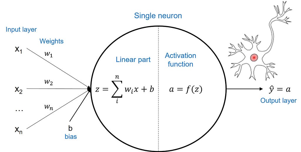
Weights assigned to input signals represent the importance of each individual signal. The neuron summarises the inputs and their weights into a linear function z, before applying an activation function a, which produces a single output (prediction).

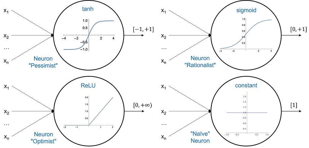
The range of output values is defined by the type of activation function. The most common activation functions are tanh (hyperbolic tangent), ReLU (rectified linear), and sigmoid functions. The image below shows these three functions in addition to one called constant, which in this case is functionally useless. Its presence is solely for fun purposes and as a memory aid. Namely, all four neurons are related to four different personalities: pessimist, rationalist, optimist, and naïve, based on the range of the functions’ values on the y-axis.

For example, the ReLU function gives only positive values ranging from zero to infinity — hence the label “optimist”. Any linear combination of weighted inputs, which results in a negative z value, gives a zero value at the output after applying the ReLU function; whilst positive z values get unchanged after applying the ReLU (as per the bottom-left image below).

The perceptron labeled as “rationalist” in the image below is Logistic Regression, which is the neural network in its most simplistic form. Its output values range from 0 to 1, hence well suited for prediction probabilities and classification tasks.

MLP Architecture

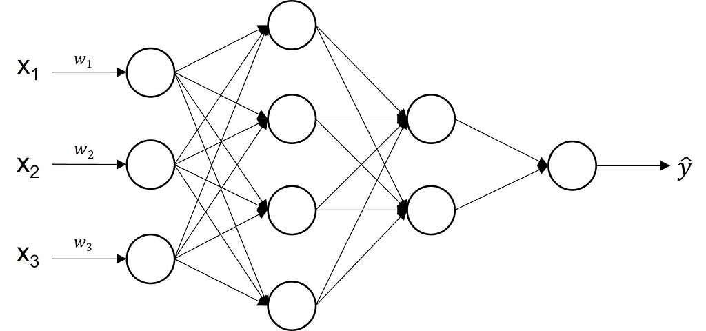
Neurons stacked together both vertically and horizontally combine to make a neural network called Multilayer perceptron. An MLP consists of an input layer, an output layer, and one or more hidden layers in between. The input layer is the plug-in for feeding the network with data, with no computation performed — it is the eyes and ears of the network. The output layer gives the model response that is prediction — a trigger for making informed decisions. A hidden layer or a feature map is a collection of neurons stacked together.

Each neuron in one layer is connected to every single neuron in the next layer, creating the fully connected layer — another synonym for MLP. But deciding how many neurons per layer and how many layers are needed is often challenging and calls for both scientific and creative solutions from data scientists. As for the number of hidden layers, the golden rule is to do more with less. So, start with the simplest network structure including logistic regression! As for the number of neurons per layer (nodes, units), a rule-of-thumb is half the number of the layer inputs.

Mathematically, MLP is a non-linear model hence, well suited for describing complex real-world problems. Each node solves a “small” problem and contributes to solving a “big” problem — resembling the human thinking process.

Convolutional Neural Network

Abbreviations: ConvNet, CNN

Filter — the Network Constituent, and Convolution Function — the Stimulus

Synonyms: filter, kernel

Filters are like lenses on a camera designed to extract and enhance special patterns (features) in images. A filter applied to image data (pixels) produces a convoluted feature map of smaller dimensions. Similarly, like perceptron, each filter solves a “small” problem and more filters orchestrated together contribute to seeing the “big picture”.

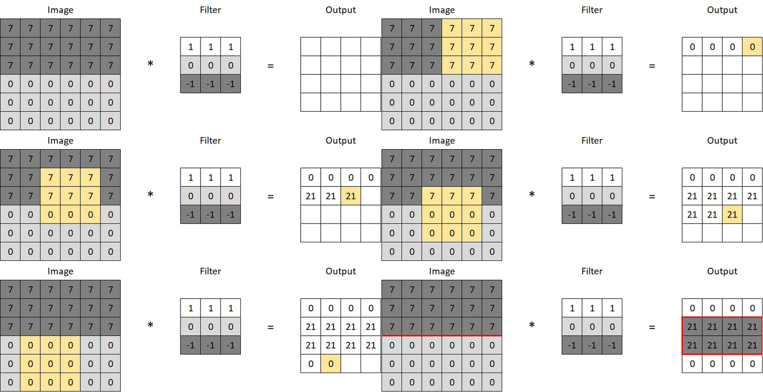
Say we want to detect the horizontal edge running through the middle of the 6×6 pixels image below. We can use a filter like the one in the same image, with some horizontally arranged numbers, indicating color intensity. We run the convolution operation (*), which scans through the image as depicted in the animated gif. At each scan, corresponding pixels of the image and the filter are multiplied (7, 0, or -7), the products are summed up (e.g. 3x7x1+3x0x0-3x7x1=0), and the results are stored in the convoluted output. The prominent horizontal line in the middle of the convoluted output below confirms the filter’s ability to recognize horizontal lines — a simple yet powerful concept.

ConvNet Architecture

ConvNets process visual data through multiple filters, channels, and layers. Filters applied to image data (i.e. pixels) produce feature maps that are convoluted layers and each map is a different version of the input image. Convolutional networks can orchestrate hundreds of filters in parallel for a single image. Image channels represent colors. Typically, we would have 3 channels per filter for each of the red, green, and blue colors.

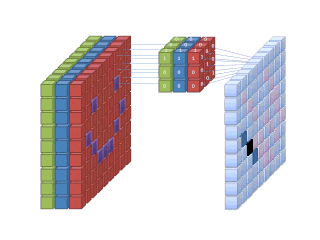
A convolutional layer has 3 dimensions: height, width, and depth. The height and width of a layer are defined by image and filter size. The layer’s depth is equal to the number of filters used to create the layer.

Hierarchically ordered layers process visual information in a feed-forward manner. The ConvNet architecture consists of different types of layers. It’s usually a combination of convolutional layers (a must have), pooling layers (a should have), and fully connected layers (a could have).

Pooling layers have multipurpose. They reduce the size of image representation, speed computation, can enhance image features, and make the ConvNet more generic and ensure the presence of an object is indifferent to the object location.

Fully connected layers (MLP layers) are usually added at the deep end of the network for image classification. For example, the final four layers of the VGG-16 network in the image below are fully connected layers. The network was trained on 1.3M images and can recognize a thousand different objects. The network consists of an input layer (image), convolutional layers (grey), pooling layers (red), and fully connected layers (blue). The final, output layer (green) is the softmax layer with 1000 neurons, which is equivalent to the number of objects the network is trained to recognize.

Constructing these layers can be considered both a science and an art. There are many parameters and an endless number of combinations. Further, there are many constraints to consider including the number of layers, size of each layer, network shape, speed or training, accuracy, and so on. Efficient deep network architectures need experts’ knowledge, skills, and imagination to master them.

Although ConvNets were created for image recognition, they can be successfully used in 1-dimensional spaces too, such as audio and time-series data.

Like humans, neural networks learn best from their mistakes

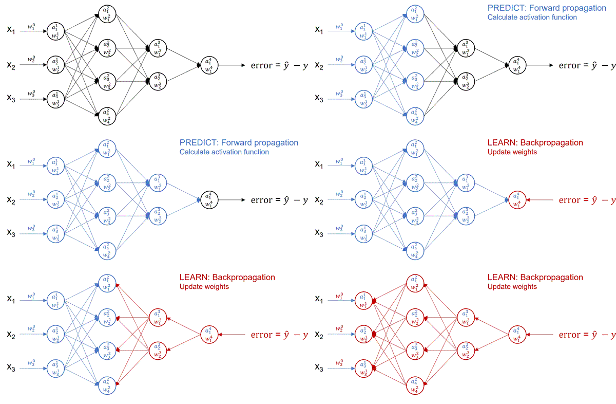
Any network is impractical unless we make it intelligent through training. The training process can resemble time traveling — it travels in the future to see the outcome (prediction). If unsatisfied, it goes back to the past, adjusts some parameters, and projects back to the future to see the new results, like in the animated image below. In this way, it keeps going forward and backward until it finds the optimal result.

In neural network terminology, this time traveling is called forward and backpropagation. Forward propagation starts by randomly assigning the weights, that is the importance of input features. It then runs from left to right, where neurons from one layer accept inputs from the previous layer, apply the activation function and pass the results to the output, which in turn becomes the input into the next layer. Forward propagation gives the prediction at the output layer. The difference between true output (y) and predicted output (y-hat) is the error or loss function. The sum of losses over the entire training examples represents the total cost function.

Cost is something we always try to minimize. In neural networks, this is achieved using the gradient descend algorithm. The objective of gradient descend is to find the network parameters that minimize the cost function. Gradient descend does this by finding descending steep slopes towards the minimum in as few steps as possible. The image below illustrates the process. In mathematical terminology, those slopes are called gradients or partial derivatives of the cost function, and they are computed during backpropagation.

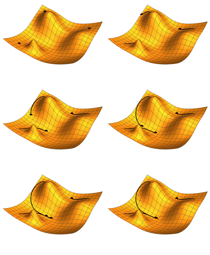
At each iteration, forward propagation feeds the prediction from left-to-right, and backpropagation feeds the loss from right-to-left and adjusts the weights, which in turn are used by forward propagation in the next iteration. At the start of model training, the loss is high as we randomly assign the weights, but it decreases at each iteration as it learns from previous mistakes! The entire process is completed once it learns which optimal weights produce the minimal cost and hence the best prediction! The weights (parameters) are what make the network intelligent — the same weights can be confidently applied to predict similar real-world problems given the new input data.

Deep Learning Frameworks

Deep learning networks can be constructed and trained using basic mathematical operations but that would be a Sisyphean task involving a great deal of calculus and algebra. Thankfully, there are specially designed frameworks, such as TensorFlow, Keras, PyTorch, and Theano that are fast, relatively simple to use, more robust, and much easier to implement in practice.

To construct a network using one of the frameworks we need to specify the number and type of layers, the number of neurons/filters per layer, the activation function, and so on. The frameworks are equipped with a set of pre-defined activation functions but also allow for custom functions, which is of special interest to the researchers. We can also specify an optimizer for minimizing the total cost function; how we want to measure the loss, that is the difference between the true value and predicted value; and what metric(s) to use for evaluating model performance. Additionally, we specify how quickly we want the cost function to reach the minimum (learning rate), set up the number of forward-backward iterations (epochs), and the number of samples for each iteration (batch size). As for batch size, we can use entire input data, a single observation, or a mini-batch for anything in between.

Using deep learning frameworks, we can control overfitting — an undesirable effect when a model performs great on training data but poorly on new (unseen) data. All these network parameters are collectively called hyperparameters and their values will vary from network to network and must be empirically set up. Hyperparameter optimization is another commodity of deep learning frameworks, which finds an optimal set of parameter values resulting in the best model performance.

Like humans, deep neural networks can share knowledge

Training complex neural network models requires time and huge computer power. The good news is that we can reuse the pre-trained models by applying them to solve similar problems and save time, resources, and lots of frustration! This is called transfer learning and is the beauty of deep learning networks.

There are many ways we can apply transfer learning. For example, we can simply remove the output layer of a pre-trained network and replace it with a new layer; or we can even replace multiple layers in the network with the new ones and train simply that portion of the network on new data.

Deep learning frameworks provide transfer learning capability. Say we want to train a network to recognize vehicles from pedestrians on images. Rather than starting from scratch, we can use a pre-trained network for image classification, such as VGG-16 from the image above, which is available in the Keras deep learning framework. We can perform this in a few simple steps: import the model, keep all its layers and their pre-trained weights, and replace only the final (green) softmax layer of 1000 neurons with another softmax layer of only 2 neurons as we only need to recognize two classes — pedestrians and vehicles. Once we have modified the network, we train the final layer only with new input images and that’s it! We have created a fast, simple, and intelligent network able to recognize vehicles from pedestrians!

Another great example of transfer learning is the ConvNet of neural style transfer [2], which produces AI art images. Specific layers of the pre-trained VGG network have been utilized for defining the style and content of AI images. Find out more about this fascinating algorithm and see some striking examples in this blog:

I wish I were van Gogh: Anything is possible with Artificial Intelligence!

Sequence Networks

Sequence networks are an esoteric concept and even attempting to go into a high level of detail on this topic would defeat the ‘keep it simple’ nature of this blog. Hence, I will only touch on some of the real-world applications of this type of network.

Sequence networks are suitable for any sequential data, where the order of data sequencing is of extreme importance. This comprises video and audio signals, time-series data, and text streams where we need to preserve and memorize the sequence orders. One such network is the recurrent neural network (RNN) of which LSTM (long-short term memory) is the most popular. One of the most prominent AI scientists and leaders in deep learning, Andrej Karpathy has expressed that:

there’s something magical about recurrent neural networks (RNNs),

as even trivial RNN structures can produce truly astonishing results!

Unlike MLPs and ConvNets, which are limited with a fixed size of inputs and outputs, sequence models do not have such constraints and both inputs and outputs can have variable lengths. For example, in sentiment analysis we have many inputs (text sequence) and only one output (a number from 1 to 5 to indicate the number of stars or smileys); in machine language translation, we have many inputs of one language, translated into many outputs of another language; or in image labeling, we have one input (an image) translated into many outputs (text description).

Attention networks are the next generation of sequence networks designed for natural language processing. Its name mimics the cognition process in which humans selectively focus their thinking. This type of network was introduced by Vaswani et. al. in their seminal paper “Attention is all you need” [3]. Popular “Alexa!”, “Okey Google!” and “Hey Siri!” are trigger word detection systems based on such networks.

Deep Great Minds

Transformers are the current state-of-the-art of deep learning networks for natural language processing, often referred to as language models. Their superiority comes from the synergy of two types of deep learning networks — attention and ConvNets. BERT [4], and T5 [5] are popular language models based on transformers networks and created by Google researchers. Both models are trained on Wikipedia and can perform various tasks including translation from one language to another, predicting the next word in a sentence (the Google search engine effectively uses it!), answering a random given question, or even creating a summary paragraph of a very long text.

The most recent breakthrough in deep learning research comes from OpenAI with two astonishing transformers — GPT-3 and DALL-E [6], the former being an AI novelist and poet and the latter an AI designer and artist. With GPT-3 you can start a novel or a poem with a few sentences or paragraphs and ask the model to complete it. DALL-E model transforms text into many images. For example, the sentence:

A loft bedroom with a white bed next to a nightstand. There is an aloe plant standing beside the bed. — OpenAI

is transformed by DALL-E into a series of images depicted below.

Pretty impressive!

References

[1] C. Szegedy, W. Liu, Y. Jia, P. Sermanet, S. Reed, D. Anguelov, D. Erhan, V. Vanhoucke and A. Rabinovich, Going deeper with convolutions (2014)

[2] A. Gatys, A. Ecker and M. Bethge, A Neural Algorithm of Artistic Style (2015)

[3] A. Vaswani, N. Shazeer, N. Parmar, J. Uszkoreit, L. Jones, A. Gomez, L. Kaiser and I. Polosukhin, Attention Is All You Need (2017)

[4] J. Devlin, M. Chang, K. Lee and K. Toutanova, BERT: Pre-training of Deep Bidirectional Transformers for Language Understanding (2019)

[5] C. Raffel, N. Shazeer, A. Roberts, K. Lee, S. Narang, M. Matena, Y. Zhou, W. Li and P. Liu, Exploring the Limits of Transfer Learning with a Unified Text-to-Text Transformer (2020)

[6] A. Ramesh, M. Pavlov, G. Goh, S. Gray, C. Voss, A. Radford, M. Chen and I. Sutskever, Zero-Shot Text-to-Image Generation (2021)

---

Deep Learning Simplified: Feel and Talk like an Expert in Neural Networks was originally published in Towards AI on Medium, where people are continuing the conversation by highlighting and responding to this story.

Join thousands of data leaders on the AI newsletter. It’s free, we don’t spam, and we never share your email address. Keep up to date with the latest work in AI. From research to projects and ideas. If you are building an AI startup, an AI-related product, or a service, we invite you to consider becoming a sponsor.

Published via Towards AI