


Building An End to End Deep Learning Model with Deployment on AWS Cloud using Amazon Sagemaker
Last Updated on July 19, 2023 by Editorial Team
Author(s): Anurag Bisht
Originally published on Towards AI.
Cloud Computing, Deep Learning
The objective of this post is to guide you through building an end to end machine learning pipeline involving deep learning and object detection using RESNET-50 architecture using AWS cloud computing service SageMaker. We will also discover how we can use Amazon Sagemaker Ground Truth to label large datasets within minutes.
The post will cover all the major aspects of the machine learning development lifecycle:
- Download the dataset of images:
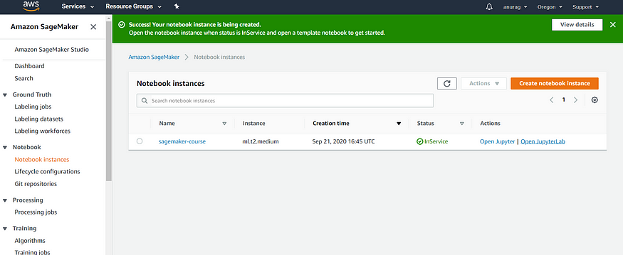
Before we even start downloading our dataset, we will spin up a sagemaker notebook instance: we can do so
- Go to your console.aws.com
- Select sagemaker service->notebook instances->create notebook instance
- Fill in the details as shown below


Jargon alert: Elastic inference: this allows GPU acceleration to increase the throughput and decrease the latency of your deep learning models.
IAM role: For someone new to cloud computing, it’s a role that provides specific permission over AWS services.
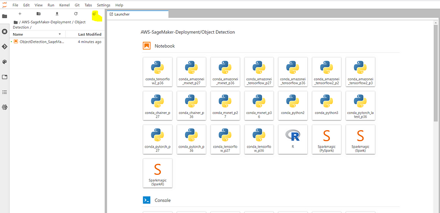
Once the instance is ready, you can open the jupyterlab notebook within the Sagemaker instance.
Once you open the Jupyterlab, you can clone the repository from this link. You will have to navigate to the object detection folder.
We will use this opensource dataset link containing 500 images of bees. So the first task would be to download the files, unzip them and upload them to the Amazon S3 bucket as amazon sagemaker uses the S3 bucket for storing artifacts.
In the Jupyter notebook write the following commands to unzip and copy the dataset along with the manifest file to the S3 bucket.
#Download & unzip the files to the ec2 instance of Amazon sagemaker
!wget http://aws-tc-largeobjects.s3-us-west-2.amazonaws.com/DIG-TF-200-MLBEES-10-EN/dataset.zip
!unzip -qo dataset.zip# S3 bucket must be created in us-west-2 (Oregon) region
BUCKET = '<Your s3 bucket name>'
PREFIX = 'input' # this is the root path to your working space, feel to use a different path#Copy the files to the s3 bucket
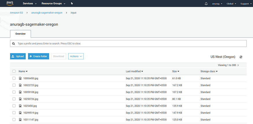
!aws s3 sync --exclude="*" --include="[0-9]*.jpg" . s3://$BUCKET/$PREFIX/

Once the data is uploaded, the respective s3 bucket will have all the images as shown below.
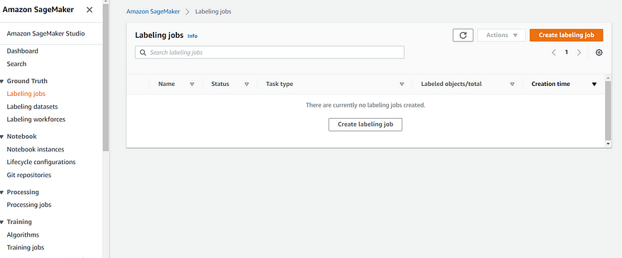
2. Using Amazon Ground Truth to create image labeling jobs
Once you have the images in the S3 bucket, you can start labeling them manually or you can use AWS powered services for automated labeling of the images. Let’s have a look that can be done.
In the labeling job section, you can create a labeling job
You can fill in the details as mentioned in the screenshot

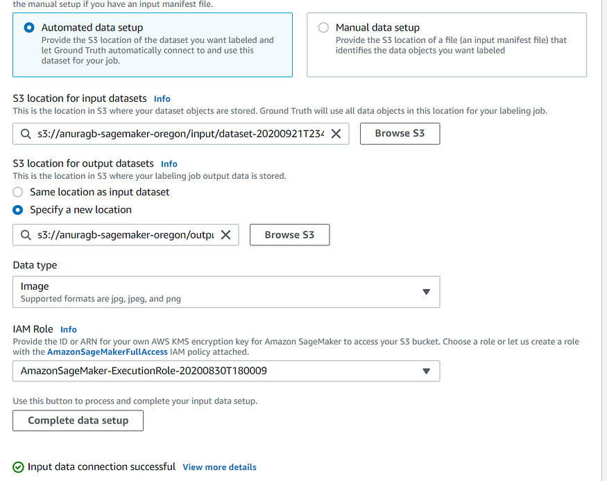
Make sure you click the complete data setup option to create a manifest file for input images. The manifest file contains all the location of dataset images in a key-value pair format. You also need to specify the IAM role for the labeling job to access the S3 bucket.
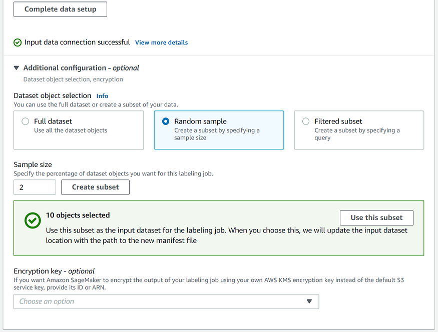
Now you can even select whether you want to label the whole dataset or sample from that dataset.
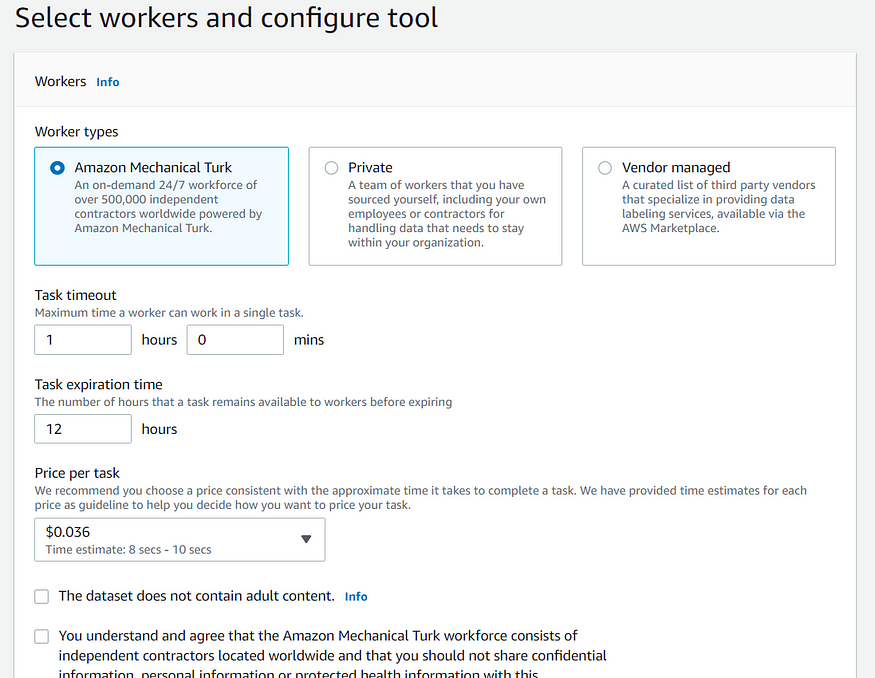
Once that's done, you need to specify the task category for the labelers.

Now you can select the type of workers for your labeling jobs: private, vendor managed, or amazon mechanical Turk (public).
Now you have to describe the label, good and bad examples.
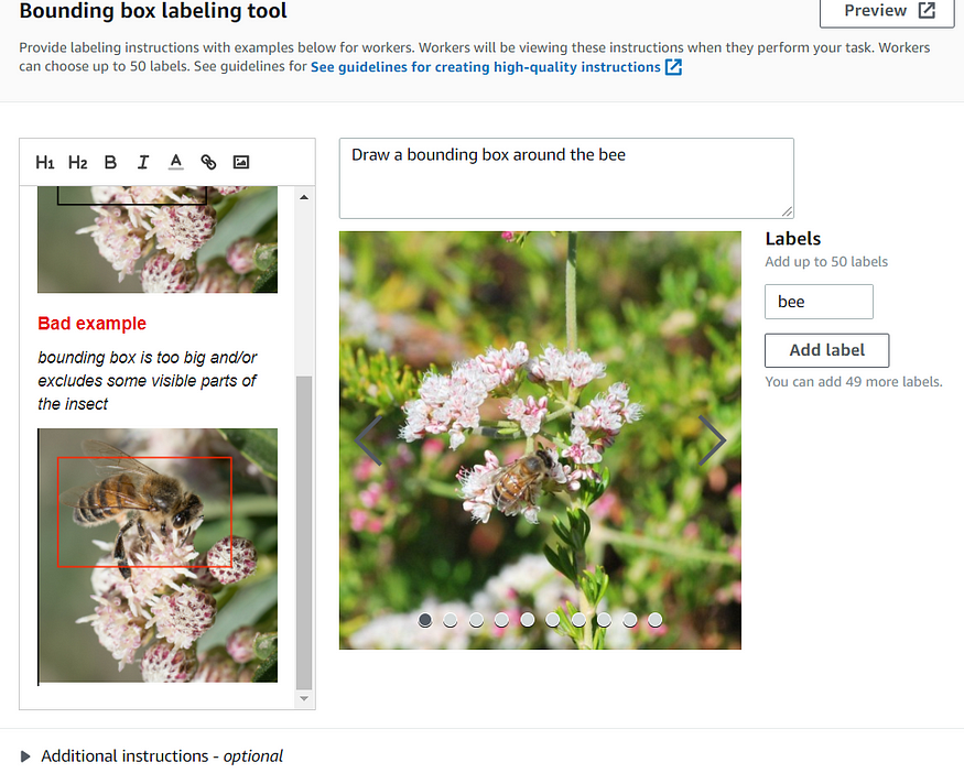
The job would look like this.

To review the annotated images we can download the manifest file with all the information about the annotation done by the labeling job.
# Enter the name of your job here
labeling_job_name = 'bees-sample'import boto3
client = boto3.client('sagemaker')s3_output = client.describe_labeling_job(LabelingJobName=labeling_job_name)['OutputConfig']['S3OutputPath'] + labeling_job_name
augmented_manifest_url = f'{s3_output}/manifests/output/output.manifest'import os
import shutiltry:
 os.makedirs('od_output_data/', exist_ok=False)
except FileExistsError:
 shutil.rmtree('od_output_data/')# now download the augmented manifest file and display first 3 lines
!aws s3 cp $augmented_manifest_url od_output_data/
augmented_manifest_file = 'od_output_data/output.manifest'
!head -3 $augmented_manifest_file#Plotting function
import matplotlib.pyplot as plt
import matplotlib.patches as patches
from PIL import Image
import numpy as np
from itertools import cycledef show_annotated_image(img_path, bboxes):
 im = np.array(Image.open(img_path), dtype=np.uint8)

 # Create figure and axes
 fig,ax = plt.subplots(1)# Display the image
 ax.imshow(im)colors = cycle(['r', 'g', 'b', 'y', 'c', 'm', 'k', 'w'])

 for bbox in bboxes:
 # Create a Rectangle patch
 rect = patches.Rectangle((bbox['left'],bbox['top']),bbox['width'],bbox['height'],linewidth=1,edgecolor=next(colors),facecolor='none')# Add the patch to the Axes
 ax.add_patch(rect)plt.show()
#Show the annotated images!pip -q install --upgrade pip
!pip -q install jsonlines
import jsonlines
from itertools import islicewith jsonlines.open(augmented_manifest_file, 'r') as reader:
 for desc in islice(reader, 10):
 img_url = desc['source-ref']
 img_file = os.path.basename(img_url)
 file_exists = os.path.isfile(img_file)bboxes = desc[labeling_job_name]['annotations']
 show_annotated_image(img_file, bboxes)
The 10 annotated images will be plotted

Before we train the model using training jobs, it’s important to split the data into training and validation parts. Here, manifest files will become handy for us to split the data sample.
import json,jsonlines
import numpy as npwith jsonlines.open('output.manifest', 'r') as reader:
 lines = list(reader)
 # Shuffle data in place.
 np.random.shuffle(lines)

dataset_size = len(lines)
num_training_samples = round(dataset_size*0.8)train_data = lines[:num_training_samples]
validation_data = lines[num_training_samples:]augmented_manifest_filename_train = 'train.manifest'with open(augmented_manifest_filename_train, 'w') as f:
 for line in train_data:
 f.write(json.dumps(line))
 f.write('\n')augmented_manifest_filename_validation = 'validation.manifest'with open(augmented_manifest_filename_validation, 'w') as f:
 for line in validation_data:
 f.write(json.dumps(line))
 f.write('\n')

print(f'training samples: {num_training_samples}, validation samples: {len(lines)-num_training_samples}')pfx_training = PREFIX + '/training' if PREFIX else 'training'
# Defines paths for use in the training job request.
s3_train_data_path = 's3://{}/{}/{}'.format(BUCKET, pfx_training, augmented_manifest_filename_train)
s3_validation_data_path = 's3://{}/{}/{}'.format(BUCKET, pfx_training, augmented_manifest_filename_validation)!aws s3 cp train.manifest s3://$BUCKET/$pfx_training/
!aws s3 cp validation.manifest s3://$BUCKET/$pfx_training/
Below would be the output for the split and once the manifest files are uploaded back to the S3 bucket.

3. Training the model using the labeled data.
There are 2 options to create training jobs:
- Using the API and code approach: The code is provided in the notebook, we will look through the console-based approach.
- Using the sagemaker console:
We will go to Sagemaker->Training Jobs->Create training job

Selecting the input mode can be subjective, you have 2 options :
File mode: your data for training will be copied to the EC2 instances where your training job starts.
Pipe mode: Your training data will be streamed in realtime to the EC2 instances.

The next step is to select the type of resource for the training job, you can select standard computing instances or GPU powered instances.
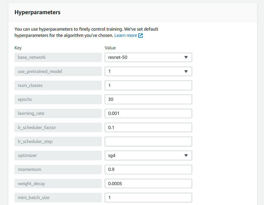
We have to specify the hyperparameters for our training jobs. The most common ones are specified in the screenshot below.
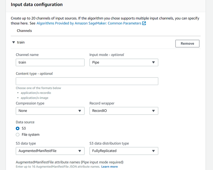
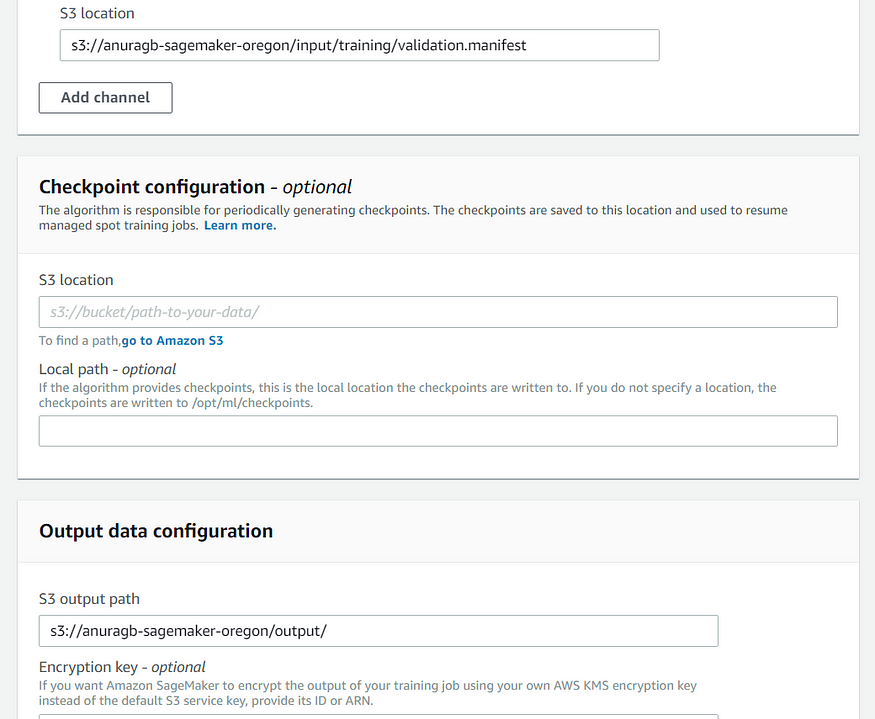
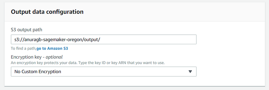
We have 2 specify 2 input configurations for training and validation channels and one output configuration for output data channel.


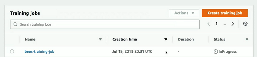
Once the training job starts you can monitor its progress.
You can also review the status of the training job programmatically through the code.
##### REPLACE WITH YOUR OWN TRAINING JOB NAME
# In the above console screenshots the job name was 'bees-detection-resnet'.
# But if you used Python to kick off the training job,
# then 'training_job_name' is already set, so you can comment out the line below.
training_job_name = 'bees-training'
##### REPLACE WITH YOUR OWN TRAINING JOB NAMEtraining_info = client.describe_training_job(TrainingJobName=training_job_name)print("Training job status: ", training_info['TrainingJobStatus'])
print("Secondary status: ", training_info['SecondaryStatus'])
4. Creation and deployment of the model
To create a model, you have to use the model artifacts created by the training job using the describe_training_job API.
import time
timestamp = time.strftime('-%Y-%m-%d-%H-%M-%S', time.gmtime())
model_name = training_job_name + '-model' + timestamptraining_image = training_info['AlgorithmSpecification']['TrainingImage']
model_data = training_info['ModelArtifacts']['S3ModelArtifacts']primary_container = {
 'Image': training_image,
 'ModelDataUrl': model_data,
}from sagemaker import get_execution_rolerole = get_execution_role()create_model_response = client.create_model(
 ModelName = model_name,
 ExecutionRoleArn = role,
 PrimaryContainer = primary_container)print(create_model_response['ModelArn'])
Before we deploy a model, we have to create an endpoint configuration. This will particularly be useful in situations where you perform a/b testing or try different variants of the models behind your endpoint.
timestamp = time.strftime('-%Y-%m-%d-%H-%M-%S', time.gmtime())
endpoint_config_name = training_job_name + '-epc' + timestamp
endpoint_config_response = client.create_endpoint_config(
 EndpointConfigName = endpoint_config_name,
 ProductionVariants=[{
 'InstanceType':'ml.t2.medium',
 'InitialInstanceCount':1,
 'ModelName':model_name,
 'VariantName':'AllTraffic'}])print('Endpoint configuration name: {}'.format(endpoint_config_name))
print('Endpoint configuration arn: {}'.format(endpoint_config_response['EndpointConfigArn']))
Once the endpoint configuration is created, you can create an endpoint either through the sagemaker dashboard or using create_endpoint API.
timestamp = time.strftime('-%Y-%m-%d-%H-%M-%S', time.gmtime())
endpoint_name = training_job_name + '-ep' + timestamp
print('Endpoint name: {}'.format(endpoint_name))endpoint_params = {
 'EndpointName': endpoint_name,
 'EndpointConfigName': endpoint_config_name,
}
endpoint_response = client.create_endpoint(**endpoint_params)
print('EndpointArn = {}'.format(endpoint_response['EndpointArn']))#check the endpoint status
endpoint_name="endpoint name from above steps"
# get the status of the endpoint
response = client.describe_endpoint(EndpointName=endpoint_name)
status = response['EndpointStatus']
print('EndpointStatus = {}'.format(status))
Once the endpoint is ready, we can perform an inference request using the below code.
#Check for the test images
import glob
test_images = glob.glob('test/*')
print(*test_images, sep="\n")def prediction_to_bbox_data(image_path, prediction):
 class_id, confidence, xmin, ymin, xmax, ymax = prediction
 width, height = Image.open(image_path).size
 bbox_data = {'class_id': class_id,
 'height': (ymax-ymin)*height,
 'width': (xmax-xmin)*width,
 'left': xmin*width,
 'top': ymin*height}
 return bbox_dataimport matplotlib.pyplot as pltruntime_client = boto3.client('sagemaker-runtime')# Call SageMaker endpoint to obtain predictions
def get_predictions_for_img(runtime_client, endpoint_name, img_path):
 with open(img_path, 'rb') as f:
 payload = f.read()
 payload = bytearray(payload)response = runtime_client.invoke_endpoint(EndpointName=endpoint_name,
 ContentType='application/x-image',
 Body=payload)result = response['Body'].read()
 result = json.loads(result)
 return result# wait until the status has changed
client.get_waiter('endpoint_in_service').wait(EndpointName=endpoint_name)
endpoint_response = client.describe_endpoint(EndpointName=endpoint_name)
status = endpoint_response['EndpointStatus']
if status != 'InService':
 raise Exception('Endpoint creation failed.')for test_image in test_images:
 result = get_predictions_for_img(runtime_client, endpoint_name, test_image)
 confidence_threshold = .2
 best_n = 3
 # display the best n predictions with confidence > confidence_threshold
 predictions = [prediction for prediction in result['prediction'] if prediction[1] > confidence_threshold]
 predictions.sort(reverse=True, key = lambda x: x[1])
 bboxes = [prediction_to_bbox_data(test_image, prediction) for prediction in predictions[:best_n]]
 show_annotated_image(test_image, bboxes)
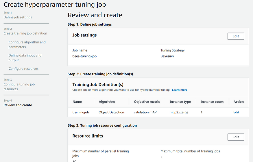
5. Hyperparameter optimization using model tuning jobs.
Although we have created and deployed our model. To improve the accuracy of our model we might have to tune the hyperparameters.
To create a hyperparameter tuning job, you can either use API or you can use the AWS console. You can either use the Bayesian optimization strategy or random search strategy.

In the job definition, the parameters are almost identical to the training job section. The only difference is that you can now select options or specify the range.

The configuration for training, validation, and output channel is given below.


Now you can configure the resources.

In the next step, you will specify the resource limits.
Once the hyperparameter job completes, you can review the job history with the best objective metric value

you can select the best combination of hyperparameters from the summary.

6. Clean up the unnecessary resources if needed
You can delete unnecessary resources or endpoints by using delete_endpoint API.
client.delete_endpoint(EndpointName=endpoint_name)
The data engineering aspect if needed in real-world use-cases is out of the scope of this post. We will definitely discuss those design principles in future posts.
We will also discuss in detail how we can use multimodel architecture behind a single endpoint, divert a portion of traffic and do A/B testing and replace the models with new production variants.
If you really enjoyed this post, then please do consider following me for good quality content and tutorials on AI/machine learning, data analytics, and BI.
Check me out on LinkedIn
Join thousands of data leaders on the AI newsletter. Join over 80,000 subscribers and keep up to date with the latest developments in AI. From research to projects and ideas. If you are building an AI startup, an AI-related product, or a service, we invite you to consider becoming a sponsor.
Published via Towards AI
Related posts


Popular posts

 for 2021")


Updates

Recent Posts


