Linear Regression Math Intuitions

Author(s): Fernando Guzman

Originally published on Towards AI.

Linear regression is the simplest model in machine learning that in its original version describes the relationship between 2 variables. It stills important to understand linear regression concepts basis, because it is the base line for understanding many other machine learning models and neural networks.

Before we dive in into linear regression workflow, let’s describe the key components or functions of this models and it’s deductions, which are listed below:

• Mean Square Error
• Prediction
• Gradient Descend

MEAN SQUARE ERROR (MSE)

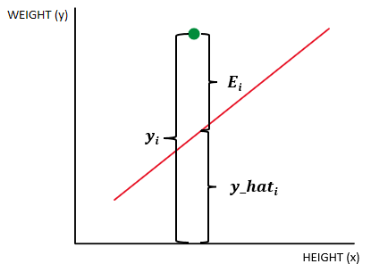
Here we are going to make the deductions for MSE which is going to be used in this model as a metric for measuring the overall model average error. So, let’s have a look at the illustration below:

Here we have yi which is the answer, y_hat which is the prediction and last there Ei which is the error respecting to the model or also known as epsilon.

From the above illustration we can deduct that the error is defined by the difference between the answer yi and the prediction y_hat, and this can be expressed as follow:

As you may have noticed, this difference is not always going to be positive because the registers or the dots in the illustration sometimes are going to be down the model function. To solve this we simple square the expression:

Once we got that, we have the expression for determining the error of a single point in the dataset, and we can extend this to express the error for the whole dataset as the following expressions, which are the same:

The formula above is the MSE itself, but it can also be expressed in a matricial form shown in the deductions below:

Keep in mind this different forms of expressing the MSE as we’ll be using any of this notations for further explanations.

PREDICTION

Our prediction is a function that builds the model essentially, which in this case is linear regression. And in this model we define the model function as the product of a vector parameters with the dataset:

Here n represents the total number of register in our dataset and D is the total size of the dataset features or also called the dimensionality size. As you can see, our parameters are going to be a vector with our dataset’s dimensionality size and we know that our dataset normally is going to be a matrix, so this expression can be simplified as follow:

Both expressions in the above illustration are completely the same.

GRADIENT DESCENT

To optimize the parameters we use gradient descent, and for this particular model we could also use a direct method which we are going to be explaining later on, for now let’s focus on the gradient descent.

The gradient descent uses the gradient of our actual error which comes to be the derivative of it, and this derivative is expressed below along with some operations we need to make to obtain the gradient:

Here, you can see that our final result is the gradient of the error respecting w which represent the parameters.

Now that we have the gradient, let’s have a look at the gradient descent expressed below:

The above formula is the original gradient descent where eta is the learning rate and the gradient of the error is what we just deducted before. Then if we replace the gradient of the error by the expression we just deducted, we get the following:

DIRECT METHOD

An alternative for the gradient descent in linear regression model is the direct method which simply consist in equal the gradient of the error expression to 0. The illustration below shows the deductions for this method:

LINEAR REGRESSION IMPLEMENTATION

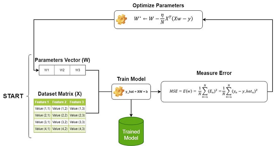
Now that we know the key methods for linear regression let’s explain its workflow with the illustration below:

As you can see, we start setting the parameters randomly and we feed it to the linear regression model along with the data, then we measure the error, and based on this we optimize the parameters using the gradient descent. We keep doing this process till the error stabilize at the minimum, then we exit this loop with our trained model with adjusted parameters. See that the parameters acts as tensors for the model.

In case of using the direct method instead of gradient descent, the adjustment of parameters will only happen once, which means that we don’t need a loop as for gradient descent.

CONSIDERATIONS

1. One thing you need to keep in mind is that the linear regression model is just the prediction and the gradient descent and the error functions are mechanisms to make a full implementation of the model and these are used in other models as well, but the model itself is the the formula that defines the prediction.
2. A second thing to consider is that in this explanation we are using the Mean Square Error as a metric to evaluate the model error, but if you wish to make a bit more research about it, you’ll find out that the Maximum Likelihood ends up being just the same for evaluating the error.

Hope this was helpful for you.

Join thousands of data leaders on the AI newsletter. Join over 80,000 subscribers and keep up to date with the latest developments in AI. From research to projects and ideas. If you are building an AI startup, an AI-related product, or a service, we invite you to consider becoming a sponsor.

Published via Towards AI