Bias-Variance decomposition 101: a step-by-step computation.

Author(s): Diletta Goglia

Originally published on Towards AI the World’s Leading AI and Technology News and Media Company. If you are building an AI-related product or service, we invite you to consider becoming an AI sponsor. At Towards AI, we help scale AI and technology startups. Let us help you unleash your technology to the masses.

Bias-variance Decomposition 101: Step-by-Step Computation.

Have you ever heard of the “bias-variance dilemma” in ML? I’m sure your answer is yes if you are here reading this article 🙂 and there is something else I’m sure of: you are here because you hope to finally find the ultimate recipe to reach the so famous best trade-off.

Well, I still don’t have this magic bullet, but what I can offer to you today in this article is a way of analyzing the error of your ML algorithm, breaking it up into three pieces, and so get a straightforward approach to understanding and concretely address the bias-variance dilemma.

We will also perform all the derivations step-by-step in the easiest way possible because without the math it is not possible to fully understand the relationship between bias and variance components and consequently take action to build our best model!

Table of content

1. Introduction and notation
2. Step-by-step computation
3. Graphical view and the famous Trade-Off
4. Overfitting, underfitting, ensemble, and concrete applications
5. Conclusion
6. References

1. Introduction and notation

In this article, we will analyze the error behavior of an ML algorithm as the training data changes, and we will understand how the bias and variance components are the key points in this scenario to choose the optimal model in our hypothesis space.

What happens to a given model when we change the dataset? How does the error behave? Imagine having and maintaining the same model architecture (e.g. a simple MLP) and assume some variation of the training set. Our aim is to identify and analyze what happens to the model in terms of learning and complexity.

This approach provides an alternative way (w.r.t. the common empirical risk approach) to estimate the test error.

What we are going to do in this article.

Given a variation of the training set, we decompose the expected error at a certain point x of the test set in three elements:

• Bias, which quantifies the discrepancy between the (unknown) true function f(x) and our hypotheses (model) h(x), averaged on data. It corresponds to a systematic error.
• Variance, quantifies the variability of the response of the model h for different realizations of the training data (changes on the training set lead to very different solutions).
• Noise because the labels d include random error: for a given point x there are more than one possible d (i.e. you are not obtaining the same target d even if sampling the same point x in input). It means that even the optimal solution could be wrong!

N.B. DO NOT CONFUSE the “bias” term used in this context with other usage of the same word to indicate totally different concepts in ML (e.g. inductive bias, bias of a neural unit).

Background and scenario

We are in a supervised learning set, and in particular, we assume a regression task scenario with target y and squared error loss.

We assume that data points are drawn i.i.d. (independent and identical distributed) from a unique (and unknown) underlying probability distribution P.

Suppose we have examples <x,y> where the true (unknown) function is

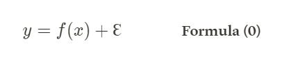
where Ɛ is Gaussian noise having zero mean and standard deviation σ.

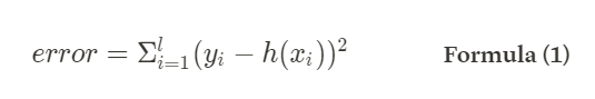
In linear regression, given a set of examples <x_i, y_i> (with i = 1, …, l) we fit a linear hypotheses h(x) = wx + w_0 such as to minimize the sum-squared error over the training data.

For the Error Function, we also provide a Python code snippet.

It’s worth pointing out two useful observations:

• Because of the hypothesis class we chose (linear) for some function f we will have a systematic prediction error ( i.e. the bias).
• Depending on the datasets we have, the parameters w found will be different.

Graphical example for a full overview of our scenario:

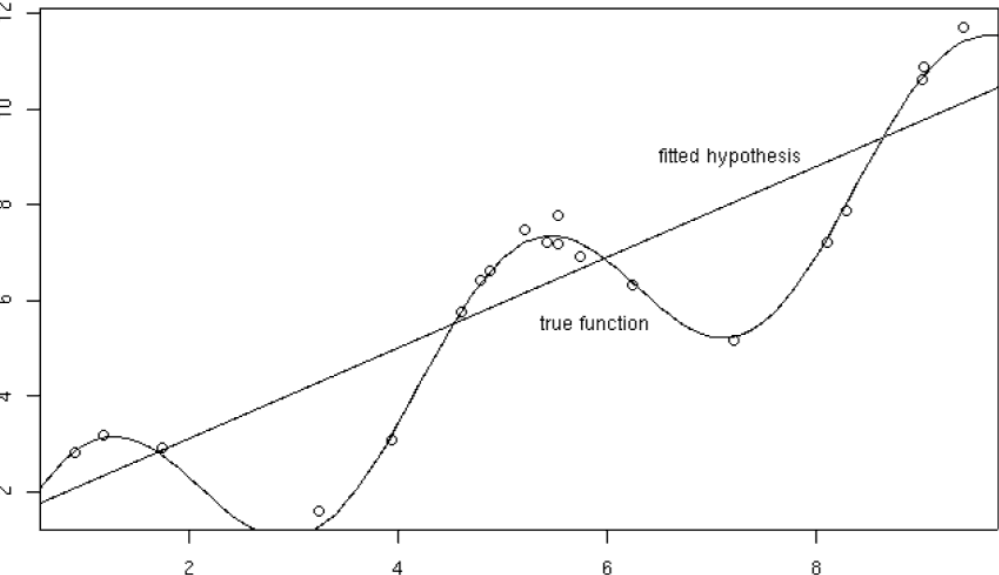
In Fig.1 it is easy to see the 20 points (dots) sampled over the true function (the curve) y = f(x) + ε. So we just know 20 points from the original distribution. Our hypothesis is the linear one that tries to approximate the data.

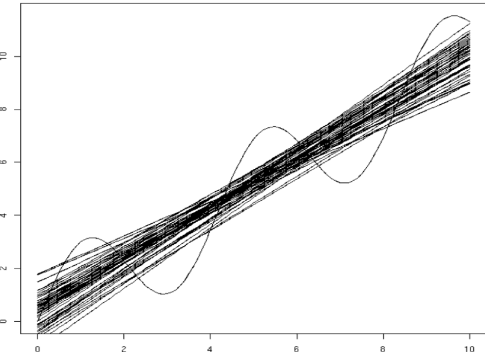
In Fig.2 we have 50 fits made by using different samples of data, each on 20 points (i.e. varying the training set). Different models (lines) are obtained according to the different training data. Different datasets lead to different hypotheses, i.e. different (linear) models.

Our point: understand how the error of the model changes according to different training sets?

Our aim

Given a new data point x what is the expected prediction error? The goal of our analysis is to compute, for an arbitrary new point x,

where the expectation is intended overall training sets drawn according to P.

Note that there is a different h (and y) for each different “extracted” training set.

We will decompose this expectation into three components as stated above, analyze how they influence the error and how to exploit this p.o.v. to set up and improve an efficient ML model.

2. Step-by-step computation

2.1 Recall basics statistics

Let Z be a discrete random variable with possible values z_i, where i = 1, …, l and probability distribution P(Z).

• Expected value or mean of Z

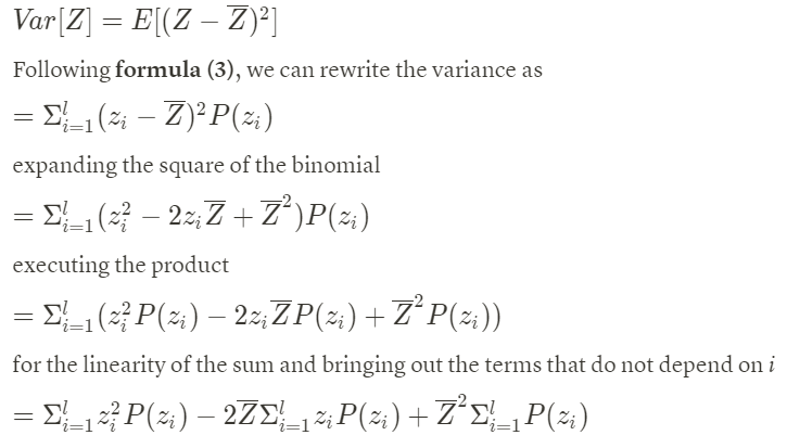
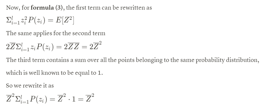
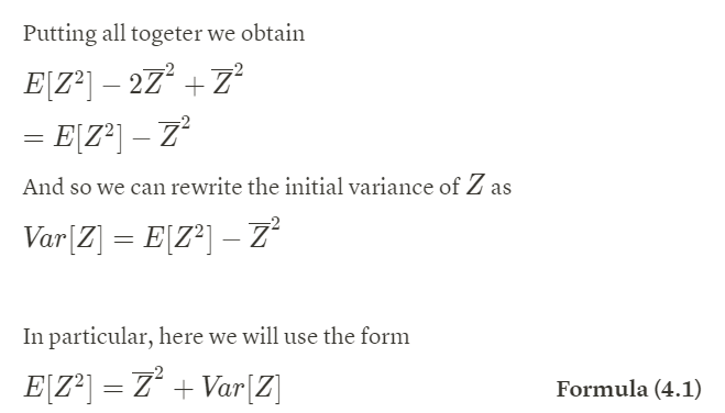
• Variance of Z

For further clarity, we will now prove this latter formula.

2.2 Proof of Variance Lemma

2.3 Bias-Variance decomposition

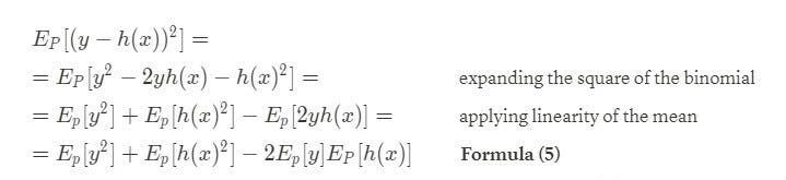
N.B. it is possible to consider the mean of the product between y and h(x) as the product of the means because they are independent variables, since, once fixed the point x on the test set, the hypothesis (model) h(x) we build the does depend (neither) on the target y (nor on x itself).

Let

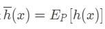
denote the mean prediction on the hypothesis at x when h is trained with data drawn from P (i.e. the mean over the models trained on all the different variations of the training set). So it is the expected value of the result that we can obtain from different training of the model with different training data, estimated at x. Now we consider each term of formula (5) separately.

Using the variance lemma (formula 4.1), we have:

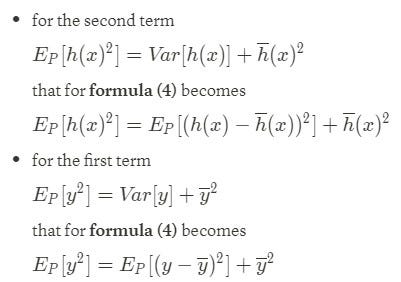
Note that, for formula (0), the expectation over the target value is equal to the target function evaluated on x:

because, by definition, the noise Ɛ has zero mean, and because the true function f(x) is assumed to be known, so the expectation over it is simply itself. For this reason, we can write:

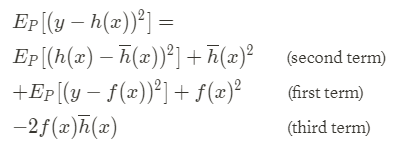
Regarding the remaining (third) term, because of, respectively, formulas (6) and (3). we can simply rewrite it as

Putting everything together and reordering terms, we can write the initial equation, i.e. formula (2):

In a compact way it is:

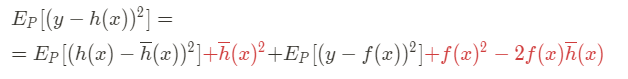
It is easy to see that the terms in red constitute a square of a binomial. Reordering again the terms for further simplicity, and rewriting in a compact way the square of the binomial:

The tree terms of formula (7) are exactly the three components we were looking for:

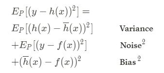
The expected prediction error is now finally decomposed in

and, since the noise has zero mean by definition — formula (0) —, we can write formula (8) : bias-variance decomposition result.

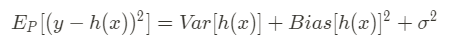
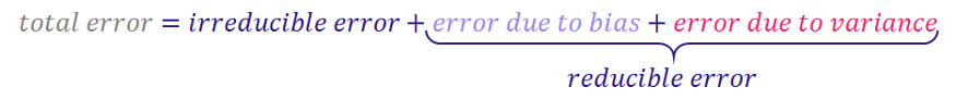
Or, following Scott Fortmann-Roe notation:

Err(x) =Bias² + Variance + Irreducible Error

Note that the noise is often called irreducible error since it depends on data and so it is not possible to eliminate it, regardless of what algorithm is used (cannot fundamentally be reduced by any model).

On the contrary, bias and variance are reducible errors because we can attempt to minimize them as much as possible.

2.4 Meaning of each term

• The variance term is defined as the expectation of the difference between each singular hypothesis (model) and the mean over all the different hypotheses (different models obtained from the different training sets).
• The bias term is defined as the difference between the mean overall the hypotheses (i.e. average of all the possible models obtained from different training sets) and the target value on the point x.
• The noise term is defined as the expectation of the difference between the target value and the target function computed on x (i.e. this component actually corresponds to the variance of the noise).

Now you have all the elements to read again the definitions of these three components given in section 1 (Introduction) and fully understand and appreciate them!

3. Graphical view and the famous Trade-Off

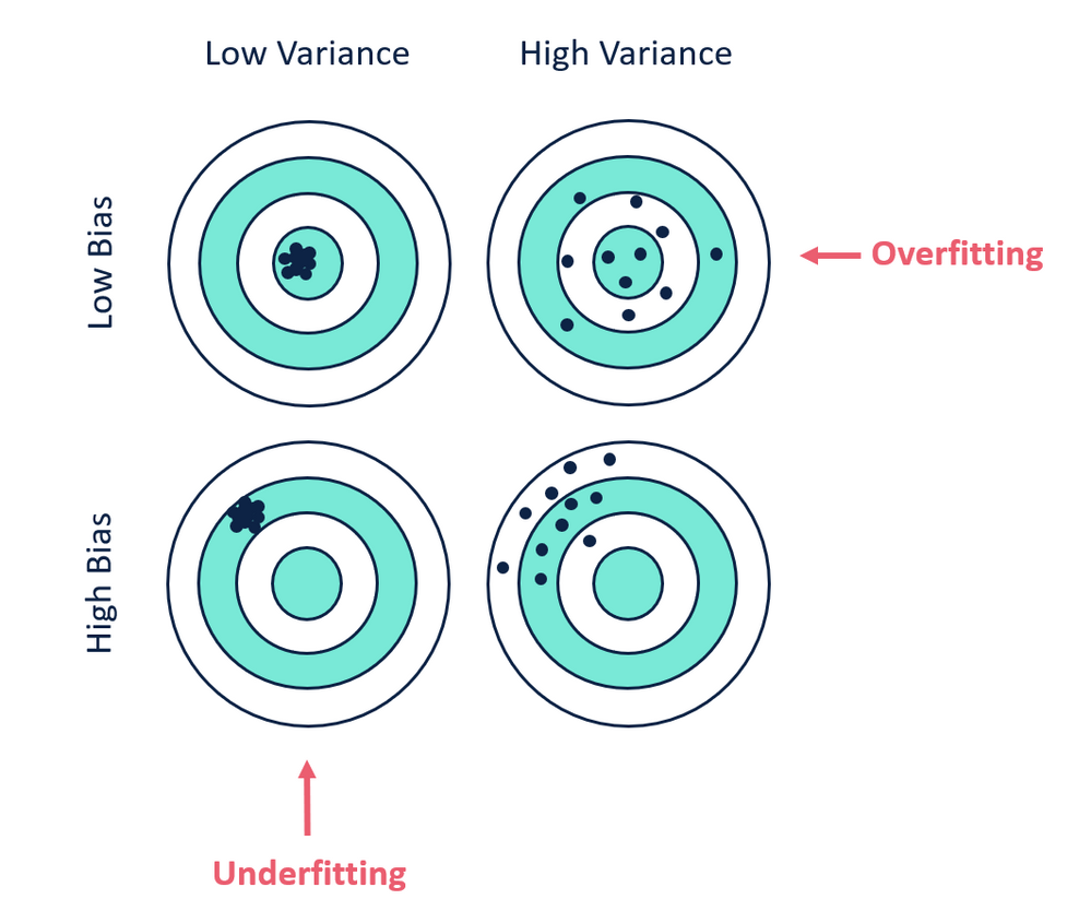
Ideally, you want to see a situation where there is both low variance and low bias, as in Fig.3 (the goal of any supervised machine learning algorithm). However, there exist often a trade-off between optimal bias and optimal variance. The parameterization of machine learning algorithms is often a battle to balance out the two since there is no escaping the relationship between bias and variance: increasing the bias will decrease the variance and vice versa.

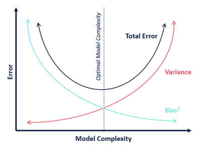
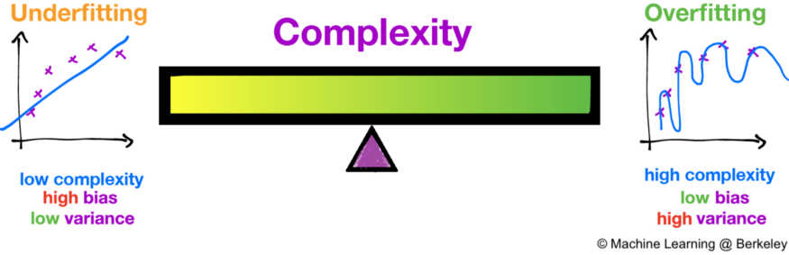
Dealing with bias and variance is really about dealing with over-and under-fitting. Bias is reduced and variance is increased in relation to model complexity (see Fig.4). As more and more parameters are added to a model, the complexity of the model rises and variance becomes our primary concern while bias steadily falls. In other words, bias has a negative first-order derivative in response to model complexity, while variance has a positive slope.

Understanding bias and variance is critical for understanding the behavior of prediction models, but in general what you really care about is an overall error, not the specific decomposition. The sweet spot for any model is the level of complexity at which the increase in bias is equivalent to the reduction in variance.

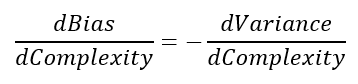
That’s why we talk about trade-offs! If one increases, the other decreases, and vice versa. This is exactly their relationship, and our derivation has been helpful to take us here. Without the mathematical expression, it is not possible to understand the connection between these components and consequently to take action to build our best model!

Let’s introduce as the last step a graphical representation of the three error components.

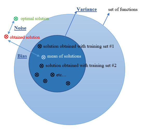
It is easy to identify:

• the bias as the discrepancy (arrow) between our obtained solution (in red) and the true solution averaged on data (in white).
• the variance (dark blue circle) as to how much the target function will change if different training data was used, i.e. the sensitivity to small variances in the dataset (how much an estimate for a given data point will change if different data set is used).

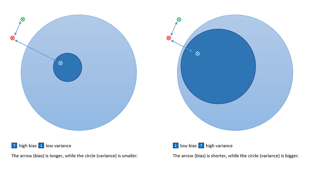
As stated before, if the bias increases the variance decreases and vice versa.

It is easy to verify graphically what we said before about the noise: since it depends on data, there is no way to modify it (that’s why it is known as irreducible error).

However, if it is true that bias and variance both contribute to error, remember that it is the (whole) prediction error that you want to minimize, not the bias or variance specifically.

4. Overfitting, underfitting, ensemble, and concrete applications

Since our final purpose is to build the best possible ML model, this derivation would be almost useless if not linked to these relevant implications and related topics:

1. Bias and Variance in model complexity and regularization. The interplay between bias-variance and lambda term in ML + their impact on underfitting and overfitting.
2. More about the famous bias-variance trade-off
3. A practical implementation to deal with bias and variance: ensemble methods.

I already covered these topics in my latest articles so if you’re interested please check them at a the links here below⬇

• Understand overfitting and underfitting in a breeze
• Overall summary of everything you can find about Bias and Variance in ML
• Ensemble Learning: take advantage of diversity.

5. Conclusion

What we have seen today is a purely theoretical approach: it is very interesting to reason about it to fully understand the meaning of each error component and to have a concrete way to approach the model selection phase of your ML algorithm. But in order to be computed, one should know the true function f(x) and the probability distribution P.

In reality, we cannot calculate the real bias and variance error terms because we do not know the actual underlying target function. Nevertheless, as a framework, bias and variance provide the tools to understand the behavior of machine learning algorithms in the pursuit of predictive performance. (Source)

I hope this article and the linked ones helped you in understanding the bias-variance dilemma and in particular in providing a quick and easy way to deal with ML model selection and optimization. I hope you will now have extra tools to approach and fix your model complexity, flexibility, and generalization capability through bias and variance ingredients.

If you enjoy this article please support me by leaving a 👏🏻. Thank you.

6. References

Main:

• Machine Learning lectures by professor A. Micheli, Computer Science master course (Artificial Intelligence curriculum), University of Pisa
• For the complete list of Medium references check this link.

Others:

• Geman, Stuart; Bienenstock, Élie; Doursat, René (1992). “Neural networks and the bias/variance dilemma” (PDF). Neural Computation. 4: 1–58. doi:10.1162/neco.1992.4.1.1.
• Vapnik, Vladimir (2000). The nature of statistical learning theory. New York: Springer-Verlag.
• Shakhnarovich, Greg (2011). “Notes on derivation of bias-variance decomposition in linear regression”
• James, Gareth; Witten, Daniela; Hastie, Trevor; Tibshirani, Robert (2013). An Introduction to Statistical Learning. Springer.
• Bias and Variance in Machine Learning — A Fantastic Guide for Beginners!, in analyticsvidhya.com
• Bias Versus Variance, in community.alteryx.com
• Understanding the Bias-Variance Tradeoff, by Scott Fortmann-Roe
• Gentle Introduction to the Bias-Variance Trade-Off in Machine Learning, in machinelearningmastery.com
• Bias–variance tradeoff, in Wikipedia

More useful sources

Bias variance decomposition calculation with mlxtend Python library:

• Calculation of Bias & Variance in python by Nallaperumal
• Bias Variance decomposition by Vidhi Chugh

More on bias-variance trade-off theory can be found in the list mentioned before.

---

Bias-Variance decomposition 101: a step-by-step computation. was originally published in Towards AI on Medium, where people are continuing the conversation by highlighting and responding to this story.

Join thousands of data leaders on the AI newsletter. It’s free, we don’t spam, and we never share your email address. Keep up to date with the latest work in AI. From research to projects and ideas. If you are building an AI startup, an AI-related product, or a service, we invite you to consider becoming a sponsor.

Published via Towards AI