How to Verify the Assumptions of Linear Regression

Author(s): Gowtham S R

Originally published on Towards AI the World’s Leading AI and Technology News and Media Company. If you are building an AI-related product or service, we invite you to consider becoming an AI sponsor. At Towards AI, we help scale AI and technology startups. Let us help you unleash your technology to the masses.

What are the assumptions of linear regression? and how to verify the assumptions

Linear regression is a model that estimates the relationship between independent variables and a dependent variable using a straight line. However, in order to use a linear regression model, we have to verify a few assumptions.

The 5 main assumptions of linear regression are,

1. A linear relationship between dependant and independent variables.
2. No/Very less multicollinearity.
3. Normality of Residuals
4. Homoscedasticity
5. No Autocorrelation of Errors

Let's understand each of the above assumptions in detail with the help of python code.

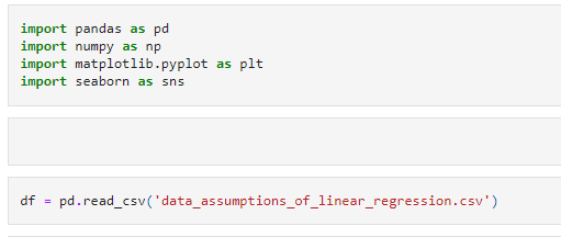
Import the required libraries, and read the dataset.

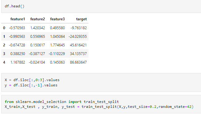
Separate the dependent and independent features, and split the data into train and test sets as shown below.

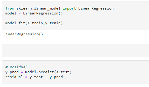
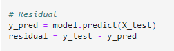
Create a linear regression model and calculate the residuals.

Let us verify the assumptions of linear regression for the above data.

1. Linear Relationship

In order to perform a linear regression, the first and foremost assumption is to have a linear relationship between the independent and the dependent features. Means — As the value of the X increases, the value of y should also increase or decrease linearly. If there are multiple independent features, each of the independent features should have a linear relationship with the dependent feature.

We can verify this assumption using a scatter plot as shown below.

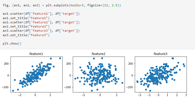
In the above scatter plots we can clearly say that features 1 and 3 are having a clear linear relationship with the target. However, feature 2 is not having a linear relationship with the target.

2. Multicollinearity

Multicollinearity is a scenario in which two of the independent features are highly correlated. So, now the question is, what is correlation? Correlation is the scenario in which two variables are strongly related to each other.

Eg, If we have a dataset where age and years_of_experience are the two independent features in our dataset. It is highly possible that as age increases, years_of_experience also increase. So, in this case, age and years of experience are highly positively correlated.

If we have age and years_left_to_retire as independent features, then as age increases, the years_left_to_retire decreases. So, here we say that the two features are highly negatively correlated.

If we have any one of the above scenarios (strong positive correlation or negative correlation), then we say that there is multicollinearity.

We can verify if there is any multicollinearity in our data, using a correlation matrix or VIF as shown in the below figure.

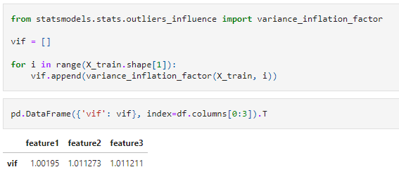
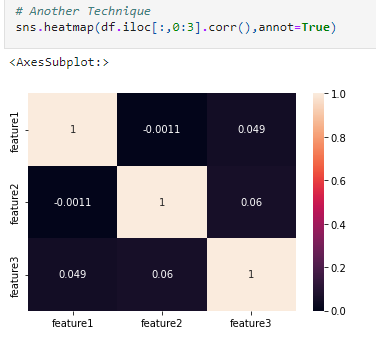
From the above VIF and correlation matrix, we can say that there is no multicollinearity in our dataset.

If you are interested in understanding multicollinearity in detail, please read my blog on why multicollinearity is a problem

Why multicollinearity is a problem?

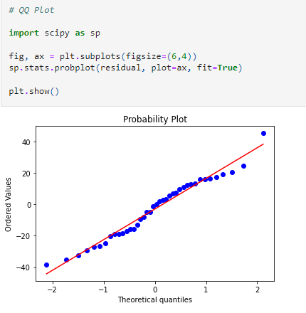
3. Normality of Residuals

Residual = actual y value − predicted y value. Having a negative residual means that the predicted value is too high, similarly, if you have a positive residual, it means that the predicted value was too low. The aim of a regression line is to minimize the sum of residuals.

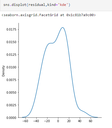
The assumption says that if we plot the residual, then the plot should be normal or sort of normal.

We can verify this assumption with the help of the KDE plot and Q-Q plot, as shown below.

4. Homoscedasticity

Homo means same and scedasticity means scatter/spread. So, the meaning of homoscedasticity is having same scatter. It means the condition in which the variance of the residual, or error term, in a regression model is constant.

When we plot the residuals, the spread should be equal. We can check this by using a scatter plot, where the x-axis will have the predictions, and the y-axis will have the residuals, as shown in the below figure.

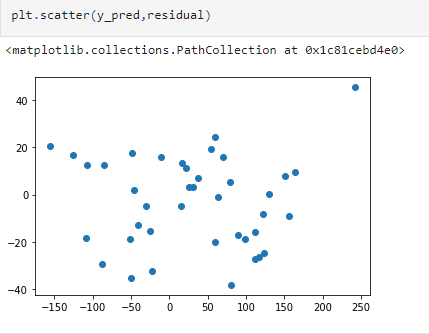
The residuals are spread uniformly, which holds the assumption of homoscedasticity.

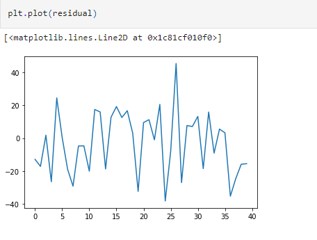
5. No autocorrelation of errors

This assumption says that there should not be any relationship between the residuals. This can be verified by plotting the residuals as shown in the below figure. The plot should not result in any particular patterns.

• Anything that can go wrong will go wrong.
• Simple ways to write Complex Patterns in Python in just 4mins.
• Which Feature Scaling Technique To Use- Standardization vs Normalization

---

How to Verify the Assumptions of Linear Regression was originally published in Towards AI on Medium, where people are continuing the conversation by highlighting and responding to this story.

Join thousands of data leaders on the AI newsletter. It’s free, we don’t spam, and we never share your email address. Keep up to date with the latest work in AI. From research to projects and ideas. If you are building an AI startup, an AI-related product, or a service, we invite you to consider becoming a sponsor.

Published via Towards AI