Supervised Contrastive Learning for Cassava Leaf Disease Classification

Last Updated on January 26, 2021 by Editorial Team

Author(s): Dimitre Oliveira

Deep Learning

Applying deep learning with supervised contrastive learning to detect diseases on cassava leaves.

Supervised Contrastive Learning (Prannay Khosla et al.) is a training methodology that outperforms supervised training with cross-entropy on classification tasks.
The idea is that training models using Supervised Contrastive Learning (SCL) can make the model encoder learn better class representation from the samples, this should lead to better generalization and robustness to image and label corruption.

In this article you will learn what is, and how supervised contrastive learn works, you will see the code implementation, an use case application and finally a comparison between SCL and regular cross-entropy.

In short, this is how SCL works:

Clusters of points belonging to the same class are pulled together in embedding space, while simultaneously pushing apart clusters of samples from different classes.

There are many contrastive learning methods like “supervised contrastive learning”, “self-supervised contrastive learning”, “SimCLR” and others, the contrastive part that they share in common is that they learn to contrast (push apart) samples that are of one domain from samples of other domains, but SCL leverages label information in a supervised way for this task.
For more detailed information check out the paper.

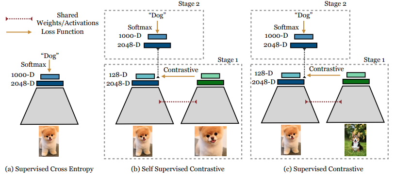
Essentially, training a classification model with Supervised Contrastive Learning is performed in two phases:

1. Training an encoder to learn to produce vector representations of input images such that representations of images in the same class will be more similar compared to representations of images in different classes.
2. Training a classifier on top of the frozen encoder.

The use case

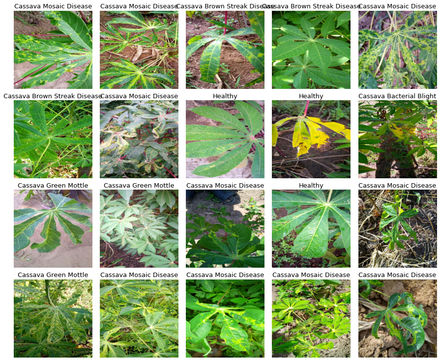
We are going to apply Supervised Contrastive Learning to a dataset from a Kaggle competition (Cassava Leaf Disease Classification) the objective is to classify images of leaves from cassava plants into 5 categories:

0: Cassava Bacterial Blight (CBB)
1: Cassava Brown Streak Disease (CBSD)
2: Cassava Green Mottle (CGM)
3: Cassava Mosaic Disease (CMD)
4: Healthy

We have four kinds of diseases and one category for healthy leaves, here are some image samples:

For more information about cassava leaf diseases, check out this link from PlantVillage.

The data has 21397 images for training and around 15000 for the test set.

Experiment set-up

— The data: Images with resolution 512 x 512 pixels.
 — The model (encoder): EfficientNet B3.
Obs: you can check the full code here.

Usually, contrastive learning methods work better if each training batch has a sample of each class, this will help the encoder learn to contrast samples of a domain from the other domains batch-wise, this means using a large batch size, and in this case, I have oversampled the minority classes, so each batch has roughly the same probability of having samples from each class.

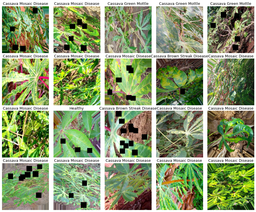
Data augmentation usually helps computer vision tasks, during my experiments I also saw improvements from data augmentation, here I am using shear, rotation, flips, crops, cutout, and changes in saturation, contrast, and brightness, it may seem a lot, but the images don’t get too different from the original ones.

Now we can look at the code

Encoder

Our encoder will be an “EfficientNet B3” but with an average pooling layer at the top of the encoder, this pooling layer will output a vector of size 2048, later it will be used to inspect the representation learned by the encoder.

def encoder_fn(input_shape):
    inputs = L.Input(shape=input_shape, name=’inputs’)
    base_model = efn.EfficientNetB3(input_tensor=inputs, 
                                    include_top=False,
                                    weights=’noisy-student’, 
                                    pooling=’avg’)
 
    model = Model(inputs=inputs, outputs=base_model.outputs)
    return model

Projection head

The projection head will be placed at the top of the encoder, and it will be responsible for projecting the output of the encoder’s embedding layer into a smaller dimension, in our case, it will project the 2048-dimension encoder into a 128-dimension vector.

def add_projection_head(input_shape, encoder):
    inputs = L.Input(shape=input_shape, name='inputs')
    features = encoder(inputs)
    outputs = L.Dense(128, activation='relu', 
                      name='projection_head', 
                      dtype='float32')(features)
    
    model = Model(inputs=inputs, outputs=outputs)
    return model

Classifier head

The classifier head is used for the optional second stage of the training, after the SCL training stage, we can remove the projection head and add this classifier head to the encoder and fine-tune the model with the regular cross-entropy loss, this should be done with the encoder’s layers frozen.

def classifier_fn(input_shape, N_CLASSES, encoder, trainable=False):
    for layer in encoder.layers:
        layer.trainable = trainable
        
    inputs = L.Input(shape=input_shape, name='inputs')
    
    features = encoder(inputs)
    features = L.Dropout(.5)(features)
    features = L.Dense(1000, activation='relu')(features)
    features = L.Dropout(.5)(features)
    outputs = L.Dense(N_CLASSES, activation='softmax', 
                      name='outputs', dtype='float32')(features)

    model = Model(inputs=inputs, outputs=outputs)
    return model

Supervised Contrastive learning loss

This is the code implementation of the SCL loss, the only parameter here is temperature, “0.1” is the default value, but it can be tweaked, larger temperatures can result in classes more separated, but smaller temperatures can benefit from longer training.

class SupervisedContrastiveLoss(losses.Loss):
    def __init__(self, temperature=0.1, name=None):
        super(SupervisedContrastiveLoss, self).__init__(name=name)
        self.temperature = temperature

    def __call__(self, labels, ft_vectors, sample_weight=None):
        # Normalize feature vectors
        ft_vec_normalized = tf.math.l2_normalize(ft_vectors, axis=1)
        # Compute logits
        logits = tf.divide(
            tf.matmul(ft_vec_normalized, 
                      tf.transpose(ft_vec_normalized)
            ), temperature
        )
        return tfa.losses.npairs_loss(tf.squeeze(labels), logits)

“tfa” is the alias for the Tensorflow addons package.

The training

I will skip the Tensorflow boilerplate training code because it is pretty standard, but you can check the complete code in this notebook.

First stage training (encoder + projection head)

The 1st stage training is done with the encoder + the projection head, using the supervised contrastive learning loss.

Building the model

with strategy.scope(): # Inside a strategy because I am using a TPU
  encoder = encoder_fn((None, None, CHANNELS)) # Get the encoder
  encoder_proj = add_projection_head((None, None, CHANNELS),encoder)
  # Add the projection head to the encoder

encoder_proj.compile(optimizer=optimizers.Adam(lr=3e-4), 
                    loss=SupervisedContrastiveLoss(temperature=0.1))

Training

model.fit(x=get_dataset(TRAIN_FILENAMES, 
                        repeated=True, 
                        augment=True), 
          validation_data=get_dataset(VALID_FILENAMES, 
                                      ordered=True), 
          steps_per_epoch=100, 
          epochs=10)

Second stage training (encoder + classifier head)

For the 2nd stage of the training, we remove the projection head and add the classifier head at the top of the encoder, which now has trained weights. For this step, we can use regular cross-entropy loss and train the model as usual.

Building the model

with strategy.scope():
    model = classifier_fn((None, None, CHANNELS), N_CLASSES, 
                          encoder, # trained encoder
                          trainable=False) # with frozen weights

    model.compile(optimizer=optimizers.Adam(lr=3e-4),
                  loss=losses.SparseCategoricalCrossentropy(), 
                  metrics=[metrics.SparseCategoricalAccuracy()])

Training
Pretty much the same as before

model.fit(x=get_dataset(TRAIN_FILENAMES, 
                        repeated=True, 
                        augment=True), 
          validation_data=get_dataset(VALID_FILENAMES, 
                                      ordered=True), 
          steps_per_epoch=100, 
          epochs=10)

Visualizing the embeddings outputs

One interesting way of evaluating the learned representation of the encoder is to visualize the output of the feature embedding, in our case, it is the last layer of the encoder, which was the average pooling layer.
Here we will be comparing the model trained with SCL with another one trained with regular cross-entropy, you can see the complete training in the reference notebook.
The visualizations are generated by applying t-SNE at the embedding outputs of the validation dataset.

Cross-entropy embedding

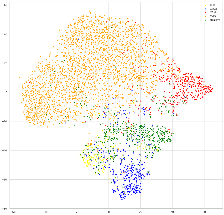
Supervised Contrastive Learning embedding

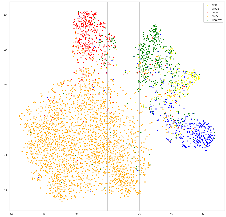
We can see that both models seem to do a good job at clustering samples of each class together, but looking at the embeddings of the model trained with SCL, the samples of each class are clustered much more apart than samples of the other classes, this is the result of the contrastive learning, we can also expect that this behavior will lead to better generalization since the classes decision boundaries will be more clear, one intuitive exercise to understand this advantage, is trying to draw the decision boundaries lines to separate the classes at each embedding, you will have a much easier time with the SCL embedding.

Conclusion

We saw that training using the supervised contrastive learning methodology is both easy to implement and efficient, it can lead to better accuracy, and better class representations, which in turn can also result in more robust models able to better generalize.
If you are willing to give SCL a try, make sure to check out the links below.

References

– Supervised Contrastive Learning paper.
– SCL paper review (video by Yannic Kilcher).
– SCL tutorial at the official Keras repository.
– SCL used on Cassava Leaf Disease Classification (Kaggle competition).
– SCL discussion thread (Kaggle competition).

Acknowledgments:

• Paper authors: Authors: Prannay Khosla, Piotr Teterwak, Chen Wang, Aaron Sarna, Yonglong Tian, Phillip Isola, Aaron Maschinot, Ce Liu, Dilip Krishnan.
  – Keras tutorial: Khalid Salama.

If you wanna check out how to build a training pipeline for computer vision using Tensorflow check out this article: “Efficiently using TPU for image classification”.

---

Supervised Contrastive Learning for Cassava Leaf Disease Classification was originally published in Towards AI on Medium, where people are continuing the conversation by highlighting and responding to this story.

Published via Towards AI