Plant Disease Detection using Faster R-CNN

Last Updated on September 6, 2020 by Editorial Team

Author(s): Amrith Coumaran

Deep Learning

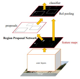
Faster R-CNN was first introduced in 2015 and is also a part of the R-CNN family. Compared to its predecessor, Faster R-CNN proposes a novel Region Proposals Network (RPN) and provides better performance and computational efficiency. The whole algorithm can be summarized by merging an RPN (region proposal algorithm) and Fast R-CNN (detection network) into a single network by sharing their convolution features. The paper states that by sharing convolutions at test-times, the cost of computing proposals is as small as 10ms per image. This post gives a brief introduction to the Faster R-CNN algorithm and implementing it to detect leaf diseases.

Region Proposal Network

An RPN is a fully convolutional network that simultaneously predicts object bounds and objectness scores at each position.

The RPN network starts by taking the output of a convolutional base network (size: H x W), which is fed with an input Image (resized to a specific size). The output of the convolutional layer depends on the stride of the neural network. In the paper, ZF-net and VGG-16 architectures are used as a base network and both have a stride of 16.

To generate region proposals, a sliding window is used over the convolutional feature map output by the last shared network layer. For every point in the feature map, the RPN has to learn whether an object is present and its dimensions and location in the input image. This is done by “Anchors”. An anchor is centered at the sliding window and is associated with the scale and aspect ratio. The paper uses 3 scales and 3 aspect ratios, yielding k = 9 anchors at each sliding window.

Now, a 3 x 3 convolution with 512 units is applied to the backbone feature map as shown in Figure 1, to give a 512-d feature map for every location (256-d for ZF and 512-d for VGG). This is fed into two sibling fully connected layers: an object classifier layer, and a bounding box regression layer.

The classifier layer is used to give probabilities of whether or not each point in the backbone feature map (size: H x W) contains an object within all 9 of the anchors at that point. So, it has 2k scores.

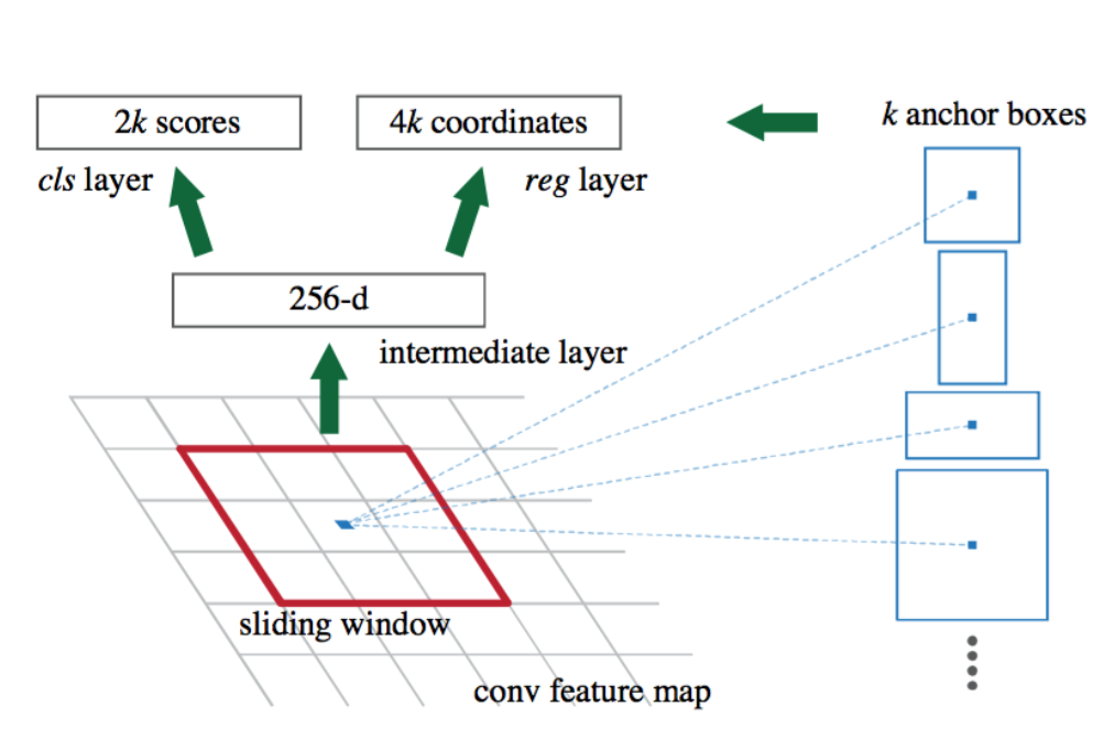
The regression layer is used to give the 4 regression coefficients of each of the 9 anchors for every point in the backbone feature map (size: H x W). So, it outputs 4k scores. These regression coefficients are used to improve the coordinates of the anchors that contain objects.

Training

Typically, the output feature map consists of about 40 x 60 locations, corresponding to 40*60*9 = 20k anchors in total. At train time, all the anchors that cross the boundary are ignored so that they do not contribute to the loss. This leaves about 6k anchors per image.

An anchor is considered to be a “positive” sample if it satisfies either of the two conditions, first, the anchor has the highest IoU (Intersection over Union, a measure of overlap) with a ground-truth box and second, the anchor has an IoU greater than 0.7 with any ground-truth box. A single ground-truth box may assign positive labels to multiple anchors.

An anchor is “negative” if its IoU with all ground-truth boxes is less than 0.3. The remaining anchors do not contribute to RPN training.

The RPN is trained end to end by backpropagation and SGD. Each mini-batch is taken from a single image that contains many positive and negative samples. We randomly sample 256 anchors in an image to compute the loss function of the mini-batch, where the sampled positive and negative anchors have a ratio of 1:1. Padding is done with negative samples if there are fewer than 128 positive samples in an image.

Detector network(Fast R-CNN):

The input image is first passed through the base network to get the feature map. Next, the bounding box proposals from the RPN are used to pool features from the backbone feature map. This is done by the ROI pooling layer. The ROI pooling layer, in essence, works by a) Taking the region corresponding to a proposal from the backbone feature map; b) Dividing this region into a fixed number of sub-windows; c) Performing max-pooling over these sub-windows to give a fixed size output. After passing them through two fully connected layers, the features are fed into the sibling classification and regression branches.

These classification and detection branches are different from those of the RPN. Here the classification layer has C units for each of the classes in the detection. The features are passed through a softmax layer to get the classification scores the probability of a proposal belonging to each class. The regression layer coefficients are used to improve the predicted bounding boxes. All the classes have individual regressors with 4 parameters each corresponding to C*4 output units in the regression layer.

The paper proposes a 4-step training algorithm to learn shared features via alternating optimization.

In the first step, the RPN is trained independently. The backbone CNN for this task is initialized with weights from a network trained for an ImageNet classification task and is then fine-tuned for the region proposal task.

In the second step, the Fast R-CNN detector network is also trained independently. The backbone CNN for this task is initialized with weights from a network trained for an ImageNet classification task and is then fine-tuned for the object detection task. At this point, they do not share the convolutional layers.

Third Step, the RPN is now initialized with weights from this Faster R-CNN detection network and fine-tuned for the region proposal task. This time, weights in the common layers between the RPN and detector remain fixed, and only the layers unique to the RPN are fine-tuned.

Finally, using the new RPN, the Fast R-CNN detector is fine-tuned. Again, only the layers unique to the detector network are fine-tuned and the common layer weights are fixed. As such, both networks share the same convolutional layers and form a unified network.

Implementation:

Clone the Github repository:

ILAN-Solutions/leaf-disease-using-faster-rcnn

$ git clone https://github.com/ILAN-Solutions/leaf-disease-using-faster-rcnn.git

$ cd leaf-disease-using-faster-rcnn

And install the packages required using,

$ pip install -r requirements.txt

Data Pre-processing:

Download the dataset here.

The Dataset has both images and its respective annotated XML files. So the following code generates a text document in the format:

img_location, x1, x2, y1, y2, class

where “img_location” is the location of the image in the directory, “x1, y1” are x-min and y-min coordinates of the bounding box respectively, “x2, y2” are x-max and y-max coordinates respectively and class is the name of the class to which the object belongs to.

Run the following code after copying your images and their respective XML files in the “train_dir” folder.

$ data_preprop.py --path train_dir --output train.txt

Training:

You can get the official faster R-CNN repository as a base code. But I have made a few changes/corrections in the validation code and added a video detection code in my GitHub repository.

I have trained my model using google colab and can find further instructions in the “leaf_disease_detection_fasterRCNN_colab.ipynb” python notebook if you are using google colab.

Run the following code for training with data augmentation.

$ python train_frcnn.py -o simple –p train.txt -hf -rot -num_epochs 50

The default parser is the pascal VOC style parser, so change it to simple parser with –o simple. Data augmentation can be applied by specifying — hf for horizontal flips, — vf for vertical flips, and — rot for 90-degree rotations.

Testing and Validation:

To run tests on the Validation set and get the output score for each image in the validation set. First, use the data_preprop.py to generate a validation.txt file. And run the measure_map.py as given below.

$ python data_preprop.p --path validation_dir --output validation.txt

$ python measure_map.py -o simple -p validation.txt

test_frcnn.py will use the trained model on a folder of images in the test directory and the output results get stored at the ‘results_imgs’ folder.

$ python test_frcnn.py -p test_dir 

video_frcnn.py will use the trained model on a video and the output video gets stored at video_results.

$ python video_stream.py -p video_test.mp4

References:

1) https://github.com/kbardool/keras-frcnn

2) Shaoqing Ren, Kaiming He, Ross Girshick, and Jian Sun, Faster R-CNN: Towards Real-Time Object Detection with Region Proposal Networks(2015), Advances in neural information processing systems.

3) Ross Girshick, Fast R-CNN(2015), Proceedings of the IEEE international conference on computer vision.

Thanks for Reading,

Amrith Coumaran

• ILAN Solutions
• amrithc – Overview

---

Plant Disease Detection using Faster R-CNN was originally published in Towards AI — Multidisciplinary Science Journal on Medium, where people are continuing the conversation by highlighting and responding to this story.

Published via Towards AI