Beginner’s guide to Timeseries Forecasting with LSTMs using TensorFlow and Keras

Last Updated on November 20, 2020 by Editorial Team

Author(s): Sanku Vishnu Darshan 

A-Z explanation of the usage of Timeseries Data for forecasting

Hello, everyone. I welcome you to the Beginner’s Series in Deep Learning with TensorFlow and Keras. This guide will help you understand the basics of TimeSeries Forecasting. You’ll learn how to pre-process TimeSeries Data and build a simple LSTM model, train it, and use it for forecasting.

What is a TimeSeries Data?

Consider you’re dealing with data that is captured in regular intervals of time, i.e., for example, if you’re using Google Stock Prices data and trying to forecast future stock prices. We capture these prices every day at successive intervals. Hence it can be termed as Timeseries Data.

To make you understand better and know in-depth about how to pre-process data, split the data into train and test, define a model and make predictions, we’ll kick start using simple Sine wave data as training data, train a deep learning model and use it to forecast values.

How does Recurrent Neural Networks work?

From a mathematical perspective, we can coin Deep Learning as a method that maps one type of variable to another type of variable using differentiable functions.

For example, If you’re performing regression, it maps the vector to a floating-point number. Similarly, if you’re dealing with a classification problem, then it could be a vector to vector mapping, where the output vector could be a probability of belonging to multiple classes.

What is a Vector?

We can define a vector as a Matrix. When you feed a deep neural network with images, it converts them into a vector of the corresponding pixel values, which will pass further into feed-forward networks. Here vector represents the meaning of the image; often, it is not understood by humans.

What are the Sequences?

When you hear the word sequences, one easy example of letting you understand this concept is to consider a sentence. It comprises a sequence of words that give it a complete meaning or consider Google Stock Prices data it contains sequences of data recorded at daily intervals.

RNNs can map sequences to vectors, vectors to sequence, or sequence to sequences. Finally, if we relate it to our current time-series problem, the model takes a sequence of input data and uses it to predict the next value.

Setup

First, import the Libraries.

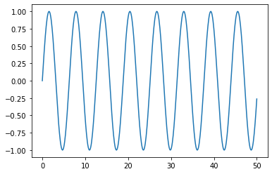
Generate the Sine Wave

We’ll use the NumPy linspace to generate x values ranging between 0 and 50 and the NumPy sine function to generate sine values to the corresponding x. Finally, let’s visualize the data.

Train, Test Split

So rather than splitting the data into train and test datasets using the traditional train_test_split function from sklearn, here we’ll split the dataset using simple python libraries to understand better the process going under the hood.

First, we’ll check the length of the data frame and use 10 percent of the training data to test our model. Now, if we multiply the length of the data frame with test_percent and round the value (as we are using for indexing purpose), we’ll get the index position, i.e., test_index. Last, we’ll split the train and test data using the test_index.

Scaling

Why do we need to Scale values?

One of the most crucial steps in data pre-processing is to scale the values. Just in case you’re an absolute beginner to Machine learning and Deep Learning, I’ll explain it to you with an easy example. For example, consider the scenario where you need to predict BMI (Body Mass Index) given the height and weight of the person. So, the values given in the height differ from weight by order of magnitude and units because height is measured in cm, whereas weight is measured in Kg. Suppose you’re using the K-Nearest Neighbour algorithm (again, the K-Nearest Neighbour algorithm works on the principle of Euclidean Distance) and plot these values. The plotted points are far away from each other, which may not help our algorithm to perform predictions.

Scenario 2: Consider if we want to use the very basic Linear Regression algorithm. It works on the principle of gradient descent, i.e., we need to find the local minima of a differentiable function. If we plot the values performing no scaling techniques, then you may end up with crazy predictions.

Scenario 3: Similarly, if you’re using an images dataset, then you need to perform unit scaling where the pixels values get normalized between 0 to 1.

To recapitulate, perform scaling normalizes the features between a definitive range.

Using Keras TimeseriesGenerator

One problem we’ll face when using Time series data is, we must transform the data into sequences of samples with input and output components before feeding it into the model. We should select the length of the sequence data in such a way so that the model has an adequate amount of input data to generalize and predict, i.e., in this situation, we must feed the model at least with one cycle of sine wave values.

The model takes the previous 50 data points (one cycle) as input data and uses it to predict the next point. This process is time-consuming and difficult if we perform this manually. Hence we’ll make use of the Keras Timeseries Generator, which transforms the data automatically and ready to train models without heavy lifting.

We can see that the length of the scaled_train is 451 and the length of the generator is 401(451–50), i.e., if we perform the tuple unpacking of the generator function using X,y as variables, X comprises the 50 data points from start and y contains the 51st data point which model uses for prediction.

Simple RNN

The variable (n_features) defined stands for the number of features in the training data, i.e., as we are dealing with univariate data, we’ll only have one feature, whereas if we are using data containing multiple features then we must specify the count of features in our data.

Test the Model

Let’s test our model using first_eval_batch. The first_eval_batch contains the last 50 points of the scaled training data and uses these to make a prediction. The results of the predicted value and the first observation in the scaled_data is commented on above for understanding. Our model predicts the next point as 0.927, whereas the original value is 0.949. Thus we can say that our model is pretty much-done training.

We can automate this processing by generating batches of data for evaluation from test data. We’ll define a function that does the heavy lifting for us.

Didn’t understand the function?. I’ll help you. First, we’ll define an empty list (test_predictions), so we can append the predicted values. The second step is to define (first_eval_batch), i.e., the first evaluation batch that needs to be sent into the model and reshape the batch, so it matches the input shape of our model. Our current_batch contains all the last 50 values from the training data.

Finally, we’ll define a loop that continues until it reaches the end of the test data. The predicted value gets appended to the (current_batch), and the first observation in the current_batch gets removed. i.e., our current_batch contains 50 values, of which 49 are from the training data, and the 50th value is the model predicted value which gets appended.

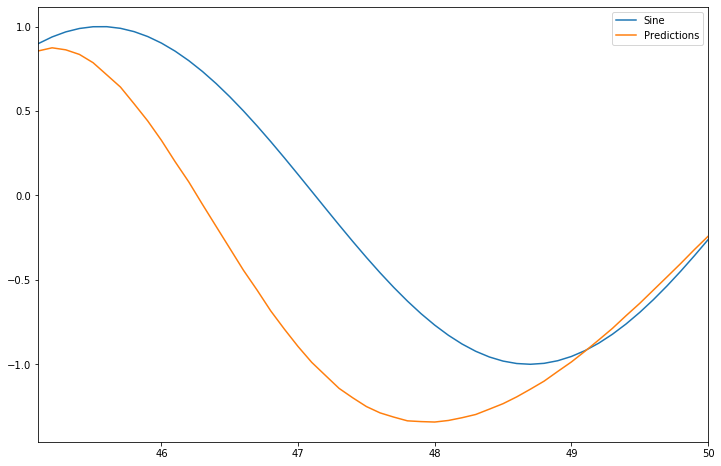
Our model does a wonderful job, right?.

There is an almost negligible difference between the predicted value and the original sine wave value at the beginning as the first batch we sent for our model evaluation comprises the last 50 values from training data; however, as the loop continues, the predicted values get appended to the batch that is fed into the model, i.e., out of 50 values 49 are from the training data and the last point the model predicted value. This process goes on until it reaches the end of test data, and as a result, more and more predicted values get appended to the evaluation batch, which may cause a slight deviation of the curve from the original values.

What are LSTMs?

An LSTM layer comprises a set of recurrently connected blocks, known as memory blocks. These blocks can be thought of as a differentiable version of the memory chips in a digital computer. Each one contains one or more recurrently connected memory cells and three multiplicative units — the input, output, and forget gates — that provide continuous analogs of write, read and reset operations for the cells. The net can only interact with the cells via the gates[1]

Again, if you are tired of these formal definitions, I’ll explain it. Consider you’re learning a new foreign language. On day one, you’ll learn some basic words like addressing a new person or saying, Hello, etc. Similarly, on day two, you’ll learn small and popular words used in day-to-day conversation. Finally, to understand and form a complete sentence in a foreign language, you must remember all the words you’ve learned so far. This is where LSTM resembles our brain. As said, they contain a ‘memory cell’ that can maintain information for lengthy periods of time. Thus LSTMs are perfect for speech recognition tasks or tasks where we have to deal with time-series data, and they solve the vanishing gradient problem seen in RNNs.

A detailed explanation of the Vanishing Gradient Problem is available in the below article.

The Vanishing Gradient Problem

LSTM

There’s no difference between the SimpleRNN model and the LSTM model, except here we’ll use LSTM Layer in a Sequential Model for our predictions.

Predictions

Visualize the Performance of Models

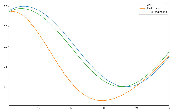
Thus we can say that LSTMs are perfect for TimeSeries Data.

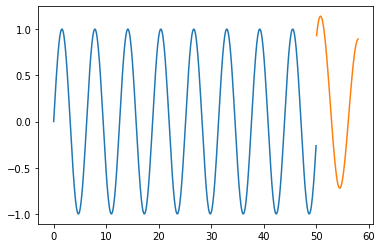
Training on Entire Data (Train+Test)

The last step or motto of building our deep learning model is to forecast values, as we had done our analysis and experimented with unique model architectures, we can conclude that LSTMs achieve high accuracy.

Thus we’ll use entire data and train the model and use them to predict the future.

Forecasting

Plot the Forecasted values

Conclusion

Congratulations! You made your first Recurrent Neural Network model! You also learned how to pre-process Time Series data, forecast into the future, something that many people find tricky.

References

1. https://machinelearningmastery.com/gentle-introduction-long-short-term-memory-networks-experts/
2. Andrej Karpathy’s Blog + Code (You can probably understand more from this now!): http://karpathy.github.io/2015/05/21/…

I hope this article has helped you to get through the basics of Recurrent Neural Networks. If you have questions, drop them down below in the comments or catch me on LinkedIn.

Until then, I’ll catch you in the next one!

---

Beginner’s guide to Timeseries Forecasting with LSTMs using TensorFlow and Keras was originally published in Towards AI — Multidisciplinary Science Journal on Medium, where people are continuing the conversation by highlighting and responding to this story.

Published via Towards AI