


How to Generate Synthetic Data?
Last Updated on January 6, 2023 by Editorial Team
Last Updated on November 15, 2020 by Editorial Team
Author(s): Fabiana Clemente
Data Science
A synthetic data generation dedicated repository
This is a sentence that is getting to common, but it’s still true and reflects the market's trend, Data is the new oil. Some of the biggest players in the market already have the strongest hold on that currency. When it comes to Machine Learning, definitely data is a pre-requisite, and although the entry barrier to the world of algorithms is nowadays lower than before, there are still a lot of barriers in what concerns the data used in real-world problems — sometimes access is restricted, others there’s not enough data to get good results, the variability is not enough for model’s generalization, and the list goes on.
For those reasons, synthetic data generation is one of the new must-have-skills for data scientists!
What is synthetic data after all?
Synthetic data can be defined as any data that was not collected from real-world events, meaning, is generated by a system with the aim to mimic real data in terms of essential characteristics. There are specific algorithms that are designed and able to generate realistic synthetic data that can be used as a training dataset. Synthetic data provides several benefits: privacy, as all the personal information has been removed, and the data is not possible to be traced back to being less costly and faster to collect when compared to collecting real-world data.
The algorithms you must know and need!
There are several different methods to generate synthetic data, some of them very familiar to data science teams, such as SMOTE or ADYSIN. Nevertheless, when it comes to generating realistic synthetic data, we shall have a look into other familiar algorithms — Deep Generative Networks. The repository I’ll be covering in this blog post is a compilation of different generative algorithms to generate synthetic data.
Generating synthetic data with WGAN
The Wasserstein GAN is considered to be an extension of the Generative Adversarial network introduced by Ian Goodfellow. WGAN was introduced by Martin Arjovsky in 2017 and promises to improve both the stability when training the model as well as introduces a loss function that is able to correlate with the quality of the generated events. Sounds good right? But what are the core differences introduced with WGAN?
What’s new in WGAN?
Instead of using the concept of “Discriminator” to classify or predict the probability of a certain generated event as being real or fake, this GAN introduces the concept of a “Critic” that in a nutshell, scores the realness or fakeness of a given event. This change is mainly due to the fact that while training a generator, theoretically we should seek the minimization of the distance between the distribution of the data observed in the training dataset and the distribution observed in the generated examples.
We can summarize the major differences introduced by WGAN as the following:
- Use a new loss function derived from the Wasserstein distance.
- After every gradient update on the critic function, clamp the weights to a small fixed range, [−c,c]. This allows for the enforcement of the Lipschitz constraint.
- An alternative proposed to the Discriminator — the Critic.
- Use of a linear activation function as the output linear of the Critic network.
- A different number of updates for the Generator and Critic Networks.
The benefits
The changes mentioned before and introduced with WGAN brings a series of benefits while training these networks:
- The training of a WGAN is more stable when compared to, for example, the original proposed GAN.
- It is less sensitive to model architecture selection (Generator and Critic choice)
- Also, less sensitive and impacted by the hyperparameters choice — although this is still very important to achieve good results.
- Finally, we are able to correlate the loss of the critic with the overall quality of the generated events.
Implementation with Tensorflow 2.0
Now what we’ve completed the imports let’s go for the networks: the Generator and the Critic.
Similarly to the Generator, I’ve decided to go for a simple Network for the Critic. Here I’ve a 4 Dense layers network with also Relu activation. But, I want to emphasize a bit here in the last code line. Different from Vanilla GAN where we add we usually add this as the last layer of the network:
x = Dense(1, activation=’sigmoid’)(x))
It uses the sigmoid function in the output layer of the discriminator, which means that it predicts the likelihood of a given event to be real. When it comes to WGAN, the critic model requires a linear activation, in order to predict the score of the “realness” for a given event.
x = Dense(1)(x)
or
x = Dense(1, activation=’linear’)(x)
As I’ve mentioned, the main contribution of the WGAN model is the use of a new loss function — The Wasserstein loss. In this case, we can implement the Wasserstein loss as a custom function in Keras, which calculates the average score for the real and generated events.
The score is maximizing the real events and minimizing the generated ones. Below the implementation of Wasserstein loss:
Another important change is the introduction of the weight clipping for the Critic Network. In this case, I’ve decided to defined to extend the Keras constraint class, with the below method:
Now that we’ve covered the major changes, you can find the full implementation of WGAN in this open GitHub repository, supported by YData.he challenges with WGAN
Although WGAN brings a lot of benefits to the area of data generation, it still has some challenges that need to be solved:
- Still suffers from unstable training, although being more stable when compared to other architectures
- Slow convergence after weight clipping — when the clipping window is too large
- Vanishing gradients — when clipping window is too small
Since its publication, and based on the fact that WGAN major issues are related to the chosen method for weights clipping, some have been the suggested improvements, being one of the most promising and used the gradient penalties — WGAN-GP article.
Tabular data generation
Now that we’ve covered the most theoretical bits about WGAN as well as its implementation, let’s jump into its use to generate synthetic tabular data.
For the purpose of this exercise, I’ll use the implementation of WGAN from the repository that I’ve mentioned previously in this blog post.
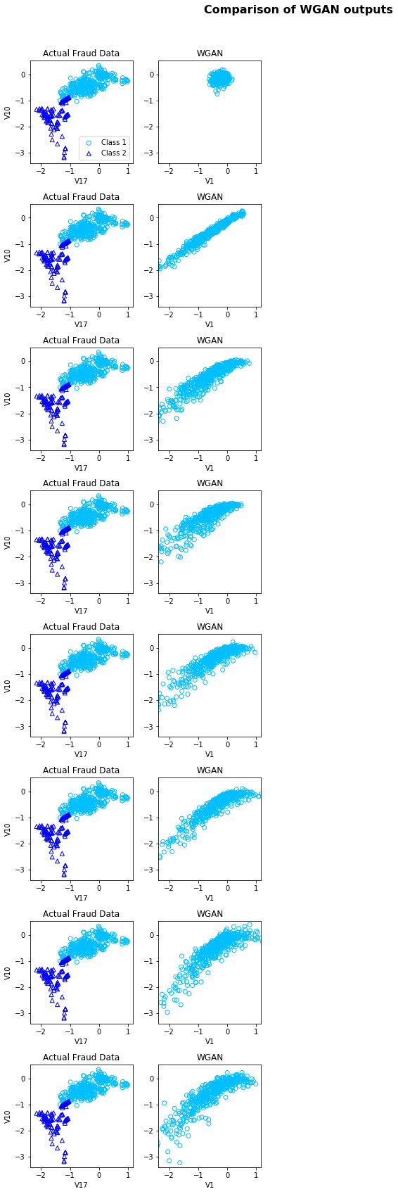
The dataset that I’ll be using for this purpose is one pretty familiar among the Data Science community — the Credit Fraud dataset.
For the purpose of demonstration, I’ve decided to go for a smaller sample of this dataset. In this case, I’ve decided to only synthesize fraudulent events.
After a few preprocessing steps on the data, we are ready to feed our data into WGAN.
Update the Critic more times than the Generator
In other GAN architectures, such as DCGAN, both the generator and the discriminator model must be updated in an equal amount of time. But this is not entirely true for the WGAN. In this case, the critic model must be updated more times than the generator model.
That’s why we have an input parameter, that I’ve called the n_critic — this parameter controls the number of times the critic gets an update from every batch of the generator. In this case, I’ve set it to 3 times. But you can set for others and check the impacts in the end results.
When compared to the training process of other GAN architectures, while using the same dataset, it is possible to perceive that indeed WGAN training was less prone to instability and producing results that are closer to the real dataset distribution, although not perfect.
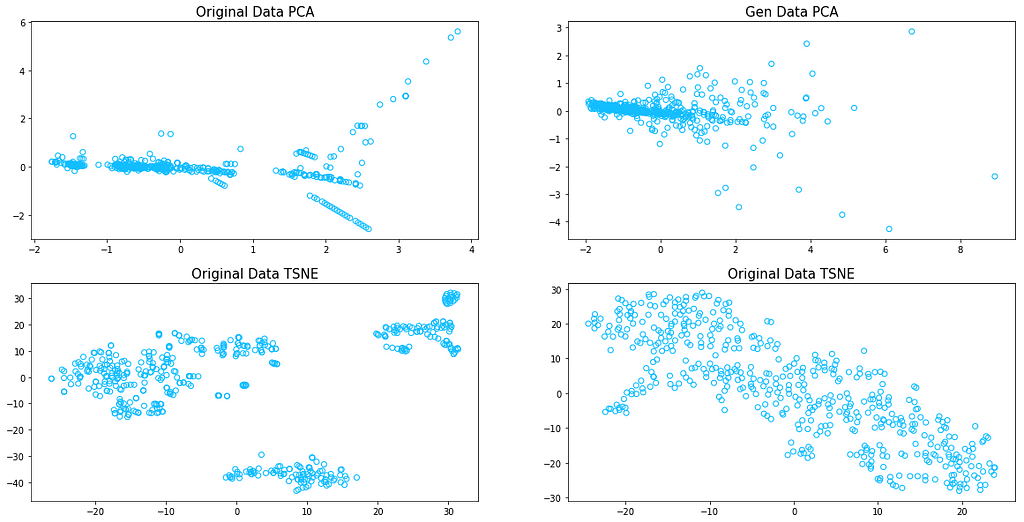
I’ve also decided to reduce the dimensionality of the dataset, by leveraging both PCA and TSNE algorithms with the choice of 2 components, in order to ease the visualization of the data. Below you can find the plots, where I compare the results of both PCA and TSNE for the WGAN generated data and the original one. It is clear, that WGAN failed to fit some of the behavior captured in the original data, nevertheless, the results are quite promising.
Conclusions
The results shown in this blog are still very simple, in comparison with what can be done and achieved with generative algorithms to generate synthetic data with real-value that can be used as training data for Machine Learning tasks.
For those who want to know more about generating synthetic data and want to have a try, have a look into this GitHub repository. We’ll be updating it with new generative algorithms as well as new dataset examples, and we invite you to collaborate!
Fabiana Clemente is CDO at YData.
Improved and synthetic data for AI.
YData provides the first dataset experimentation platform for Data Scientists.
How to Generate Synthetic Data? was originally published in Towards AI on Medium, where people are continuing the conversation by highlighting and responding to this story.
Published via Towards AI
Towards AI Academy
We Build Enterprise-Grade AI. We'll Teach You to Master It Too.
15 engineers. 100,000+ students. Towards AI Academy teaches what actually survives production.
Start free — no commitment:
→ 6-Day Agentic AI Engineering Email Guide — one practical lesson per day
→ Agents Architecture Cheatsheet — 3 years of architecture decisions in 6 pages
Our courses:
→ AI Engineering Certification — 90+ lessons from project selection to deployed product. The most comprehensive practical LLM course out there.
→ Agent Engineering Course — Hands on with production agent architectures, memory, routing, and eval frameworks — built from real enterprise engagements.
→ AI for Work — Understand, evaluate, and apply AI for complex work tasks.
Note: Article content contains the views of the contributing authors and not Towards AI.
Related posts


Recent Posts


")