


Unlocking the Power of Recurrent Neural Networks: A Beginner’s Guide
Last Updated on July 25, 2023 by Editorial Team
Author(s): Gaurav Nair
Originally published on Towards AI.
This blog covers a beginner-level introduction to Recurrent Neural Networks, forward and backpropagation through time, and its implementation in Python using NumPy.
Introduction
With the advancement of Artificial Intelligence (AI) and its practical applications in different fields, there have been a number of stepping stones that have been instrumental in the evolution of AI. The earliest applications of AI began in the late 1950s and early 1960s when researchers developed a computer program that could play simple games. From developing algorithms that could play simple games to performing advanced natural language processing tasks, such as chatGPT, many algorithms have been developed, tweaked, tried, and tested for the purpose of solving real-world problems.
Out of the many machine-learning models and neural network architectures, sequence models have proved to be a game-changer by revolutionizing the way we communicate with technology. From speech recognition to natural language processing and computer vision, sequence models find their applications in many fields today. Among the types of sequence models, the idea behind Recurrent Neural Networks(RNN) has transformed the way we process sequential data. In this article, we will see the principle behind vanilla RNNs and how it is different from conventional Artificial Neural Networks(ANN).
But what are Sequence Models?
Sequence Models are neural network architectures that process sequence data, for example, natural language, time series, or audio. They are used to predict the next item in the sequence or classify words in a particular category. Applications of Sequence Models are in Speech Recognition, Machine Translation, Music Generation, Sentiment classification, etc.
There are various Sequence models such as Recurrent Neural Networks(RNN), Gated Recurrent Units(GRU), Long-short-term Memory(LSTM), Transformers, etc. So let us understand what (vanilla)RNN is, its architecture, types, and limitations.
(Vanilla) Recurrent Neural Network
The idea of RNNs was introduced by researchers at the Massachusetts Institute of Technology(MIT) in the 1980s, and they were fully developed by the 1990s. RNN is a deep learning architecture that is designed to process sequential data. The main difference between RNN and conventional ANN is that RNN has a feedback loop that goes as input into the next time step. This way, the model is able to learn the information from previous time steps. RNN’s tweaked/improved versions have become the most powerful tool for solving a range of sequential data processing tasks.
Why do we need a Recurrent Neural Network?
(Problems with conventional ANN to work with sequence data)
Conventional ANNs have two main limitations when they are used to process sequential data. They are:
- Conventional ANNs fail to learn the features across different positions. This is why they do not do a good job while processing sequence tasks. Let us understand this with an example:
Sentence — 1: One should never tell a lie.
Sentence — 2: Doctor asked him to lie down.
The above two sentences have a common word ‘lie’, having the same spelling but different meanings. While working with text data, we convert the words to their embeddings(representation of a word). Now, it becomes essential for the model to understand the context in which this word is used in order to correctly assign it a value. - The input and output usually have the same length as the conventional ANNs. This restricts us from working with sequential data like language translation, where input and outputs can be of varied lengths.
Recurrent Neural Network Architecture
RNNs work the same way as conventional ANNs. It has weights, bias, activation, nodes, and layers. We train the model with multiple sequences of data, and each sequence has time steps. Each hidden state computes the input from the input layer and input from the previous layer. The output from the hidden state goes to the output layer and to the next hidden state.
Forward Propagation through time in RNN
While working with sequential data, the output at any time step(t) should depend on the input at that time step as well as previous time steps. This can be achieved by linking the different time steps and adding a hidden memory (internal memory or self-state) that transfers the last time step’s information. This way, we can make a network that has its output affected by what has happened in the past.
In other words, we can say that the output at any time step (ŷ sub t) is a function of input at that time step(x sub t) and the output from previous time steps(h sub t-1).

Let’s understand the computations happening at each state mathematically. Input to RNN will be in vector (x sub t), then the computation at the hidden state will be given as:

Tanh(Hyperbolic tangent) is the preferred activation function as it maps the input to output values between 1 and -1. Tanh brings non-linearity to the model, which helps compute complex decision boundaries.
Similarly, computation at the output state will be:

We can visualize computation at time step t to understand it better.

Backward Propagation through time in RNN
In a conventional neural network, Backpropagation is a training algorithm that backpropagates the derivatives of losses to update parameters. Backpropagation in RNN is a variant of this algorithm known as Backpropagation through time. Backpropagation through time allows the RNN to learn patterns that are multiple time steps away.
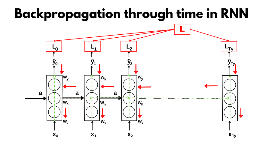
For RNNs, the forward pass through the network consists of going forward across time and then computing the losses in individual time steps. Similarly, we backpropagate errors individually across each time step and then across all the time steps. The error in each time step depends on the error at its previous time step. This is because the output at each time step depends upon the input at that step and the output of all previous time steps. This way, gradients at each step are calculated, and accordingly, the weights are updated back in time.
Let’s take the example of error/loss at timestep t2 that is L2, to understand it better. We will follow the same derivative calculation as in conventional neural networks. So at L2, through the chain rule, we can calculate the gradients to adjust the weight wy:

Similarly, we will calculate the derivatives for wh and wy. After calculating all the derivatives, we will update the weights and bias using the formula:

In a similar fashion, we will be able to update wh, wx, bh, and by. Alpha(α) is the learning rate that determines the step size while moving toward the minima.
Here’s the python code for simple RNN implementation using NumPy:
import numpy as np

class RNN:

 def __init__(self, input_size, hidden_size, output_size, learning_rate = 0.001):
 self.lr = learning_rate
 self.input_size = input_size
 self.hidden_size = hidden_size
 self.output_size = output_size

 # Weights
 self.wx = np.random.randn(input_size, hidden_size) / 1000
 self.wh = np.random.randn(hidden_size, hidden_size) / 1000
 self.wy = np.random.randn(hidden_size, output_size) / 1000

 # Biases
 self.bh = np.zeros((1, hidden_size))
 self.by = np.zeros((1, output_size))

 # Forward Propagation
 def forwardprop(self, x):

 # Initializing h with zeros
 prev_h = np.zeros((self.wh.shape[0], 1))

 for i in range(x.shape[0]):
 # Computation in the hidden state
 h = np.tanh(np.dot(x, self.wx) + np.dot(prev_h, self.wh) + self.bh)
 prev_h = h

 # Computation in the output state
 y = h * self.wy + self.by
 return y, h

 # Backpropagation through time
 def backprop(self, x, h, y, y_true):

 t = x.shape[0]

 d_wx = np.zeros_like(self.wx)
 d_wh = np.zeros_like(self.wh)
 d_wy = np.zeros_like(self.wy)
 d_bh = np.zeros_like(self.bh)
 d_by = np.zeros_like(self.by)
 d_h = np.zeros((t + 1, self.hidden_size))

 # Looping in reverse for backpropagation
 for i in range(t - 1, -1, -1):
 dy = y - y_true

 # Gradient calculation in the Outer Layer
 d_wy += np.dot(h[i].reshape(-1, 1), dy.reshape(1, -1))
 d_by += dy

 # Gradient calculation in the Hidden Layer
 d_h[i] = np.dot(self.wy.T, dy) + dh[i + 1] * (1 - np.power(h[t], 2))
 d_wh += np.dot(h[i - 1].reshape(-1, 1), dh[i].reshape(1, -1))
 d_by += d_h[i]

 # Gradient calculation in the Input Layer
 d_wx += np.dot(x[i].reshape(-1, 1), d_h[i].reshape(1, -1))

 # Updating the Weights and Biases
 self.wx -= self.lr * d_wx
 self.wh -= self.lr * d_wh
 self.wy -= self.lr * d_wy
 self.bh -= self.lr * d_bh
 self.by -= self.lr * d_by
You can also find the code on GitHub.
Types of RNN
Depending on the number of inputs and outputs RNNs can take and return; they can be divided into 5 types:
- One-to-One: A one-to-one RNN takes a single input and generates a single output. It has its application in image classification.
- One to Many: One-to-many RNN takes a single input and generates multiple outputs. Its application can be a music generator that would take only the key/scale as input and return multiple notes in the same scale as output.
- Many to One: This type of RNN takes multiple inputs and returns only one output. One of the best examples is Sentiment classification. The RNN will take the text as input which can be of varied lengths and return output as either positive or negative.
- Many to Many: Many to many RNN takes multiple inputs and returns multiple outputs. Usually, the number of inputs and outputs is the same.
- Many to Many (Encoder Decoder): There is another form of many-to-many RNN that takes multiple inputs and generates multiple outputs; however, the number of inputs and outputs is not the same. One of the popular applications of this type of RNN is machine translation.

Limitations of Recurrent Neural Network
The vanilla RNNs are not very good when it comes to capturing long-term dependencies. Languages can have long-term dependencies, so the model must capture and retain the information throughout. For example:
The artists who performed yesterday had a lot of achievements in their name and were from India.
While training the RNN models, it is seen that they fail to retain information for longer periods of time. The second word of the sentence, “artists,” is in a plural form, and hence the word “were” is used to tell about the place they belong to. For language models, it is essential that the model can capture these long-range dependencies and correctly classify singular and plural, as in this case. RNNs usually fail to retain the information till later time steps. The below diagram shows the loss of information(arrows in blue) from the first step up to the last time step.

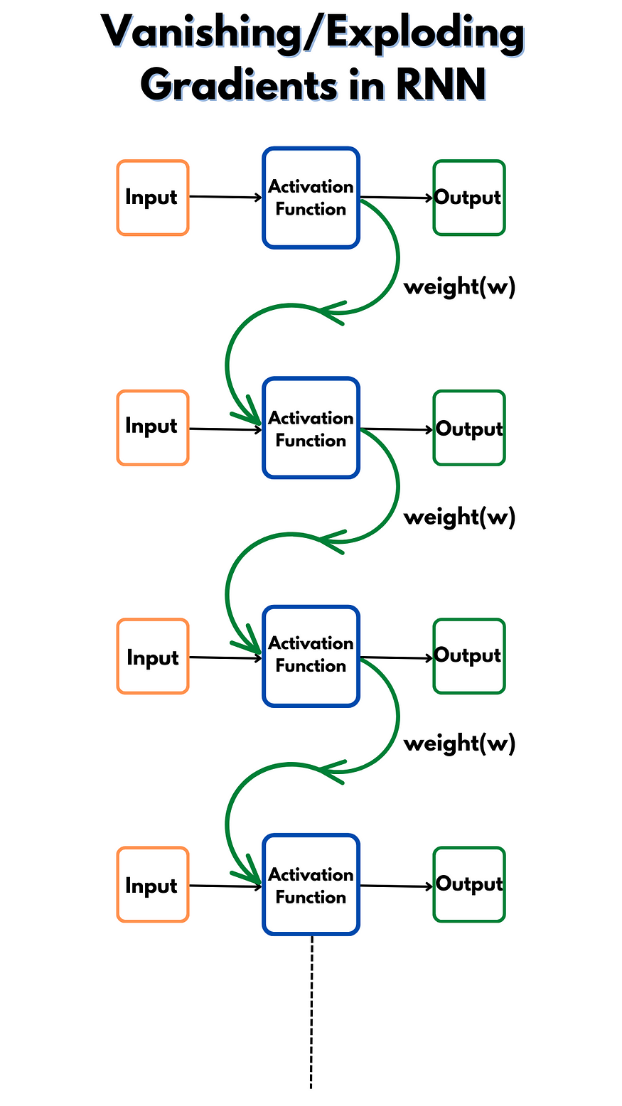
Vanishing/Exploding Gradients in RNN
One of the major drawbacks of Recurrent Neural networks is it runs into a vanishing or exploding gradient problem during backpropagation. This makes the model inefficient to learn as the weights might not update if the gradient becomes too small or increase drastically if the gradient gets too large. To understand this in a better way, let’s look at the below diagram on how it occurs. For a better understanding, let’s ignore all other weights.
While backpropagating the derivatives in RNN, we need to compute the gradient at any time step with respect to all the gradients at previous time steps. This results in repeated gradient computation. But why this results in gradient issues?
If we have weights that might be larger than 1, we will be able to see that the gradients will explode due to repeated computations. For example, if the weight is (say) 2, then at each time step, the computation will be multiple of 2(= Input * weights). If we repeat this step 5 times, then it will result in 2 to power 5. And if we have (say) 500-time steps, then weights would become 2⁵⁰⁰. Well, this will be a huge number, and while you are working on some data, you will start to see NaN values. These NaN values signify that there was a numerical overflow. This huge number will not let us take small steps to get to the minimum and reach the optimum value for weights and biases. This is called the Exploding Gradient problem.
Gradient Clipping is a solution to Exploding Gradient problem wherein we can set an upper limit so that the gradients do not become bigger than this limit. But in certain cases, clipping might result in vanishing gradients. If the value of the weights is very small, with every iteration, the gradients will start to vanish.
Conclusion
Despite all the limitations, RNNs are still used in modeling time series, audio, weather, and much more. RNN architecture is a stepping stone and has led to ideas of many advanced architectures which solve the major limitations of RNNs. Lastly, RNNs are still an active area of research, and we can expect many more architectures influenced by RNNs.
If you have made it to the end, thanks for taking the time to read the article! U+1F642
Join thousands of data leaders on the AI newsletter. Join over 80,000 subscribers and keep up to date with the latest developments in AI. From research to projects and ideas. If you are building an AI startup, an AI-related product, or a service, we invite you to consider becoming a sponsor.
Published via Towards AI
Related posts


Popular posts

 for 2021")


Updates

Recent Posts


