


")
The Basics of Recurrent Neural Networks (RNNs)
Last Updated on July 25, 2023 by Editorial Team
Author(s): Ben Khuong
Originally published on Towards AI.
Machine Learning
Table of contents
- What are RNNs used for?
- What are RNNs and how do they work?
- A trivial example — forward propagation, backpropagation through time
- One major problem: vanishing gradients
What are RNNs used for?
Recurrent Neural Networks (RNNs) are widely used for data with some kind of sequential structure. For instance, time series data has an intrinsic ordering based on time. Sentences are also sequential, “I love dogs” has a different meaning than “Dogs I love.” Simply put, if the semantics of your data is altered by random permutation, you have a sequential dataset and RNNs may be used for your problem! To help solidify the types of problems RNNs can solve, here is a list of common applications¹ :
- Speech Recognition
- Sentiment Classification
- Machine Translation (i.e. Chinese to English)
- Video Activity Recognition
- Name Entity Recognition — (i.e. Identifying names in a sentence)
Great! We know the types of problems that we can apply RNNs to, now…
What are RNNs and how do they work?
RNNs are different than the classical multi-layer perceptron (MLP) networks because of two main reasons: 1) They take into account what happened previously and 2) they share parameters/weights.
The architecture of an RNN
Don’t worry if this doesn’t make sense, we’re going to break down all the variables and go through a forward propagation and backpropagation in a little bit! Just focus on the flow of variables at first glance.
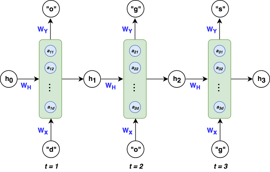
A breakdown of the architecture
The green blocks are called hidden states. The blue circles, defined by the vector a within each block, are called hidden nodes or hidden units where the number of nodes is decided by the hyper-parameter d. Similar to activations in MLPs, think of each green block as an activation function that acts on each blue node. We’ll talk about the calculations within the hidden states in the forward propagation section of this article.
Vector h — is the output of the hidden state after the activation function has been applied to the hidden nodes. As you can see at time t, the architecture takes into account what happened at t-1 by including the h from the previous hidden state as well as the input x at time t. This allows the network to account for information from previous inputs that are sequentially behind the current input. It’s important to note that the zeroth h vector will always start as a vector of 0’s because the algorithm has no information preceding the first element in the sequence.


Matrices Wx, Wy, Wh — are the weights of the RNN architecture which are shared throughout the entire network. The model weights of Wx at t=1 are the exact same as the weights of Wx at t=2 and every other time step.
Vector xᵢ— is the input to each hidden state where i=1, 2,…, n for each element in the input sequence. Recall that text must be encoded into numerical values. For example, every letter in the word “dogs” would be a one-hot encoded vector with dimension (4×1). Similarly, x can also be word embedding or other numerical representations.

RNN Equations
Now that we know what all the variables are, here are all the equations that we’re going to need in order to go through an RNN calculation:

These are the only three equations that we need, pretty sweet! The hidden nodes are a concatenation of the previous state’s output weighted by the weight matrix Wh and the input x weighted by the weight matrix Wx. The tanh function is the activation function that we mentioned earlier, symbolized by the green block. The output of the hidden state is the activation function applied to the hidden nodes. To make a prediction, we take the output from the current hidden state and weight it by the weight matrix Wy with a softmax activation.
It’s also important to understand the dimensions of all the variables floating around. In general for predicting a sequence:

Where
- k is the dimension of the input vector xᵢ
- d is the number of hidden nodes
Now we’re ready to walk through an example!
A trivial example
Take the word “dogs,” where we want to train an RNN to predict the letter “s” given the letters “d”-“o”-“g”. The architecture above would look like the following:
To keep this example simple, we’ll use 3 hidden nodes in our RNN (d=3). The dimensions for each of our variables are as follows:
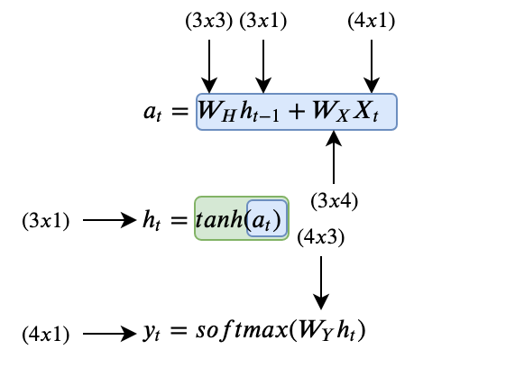
where k = 4, because our input x is a 4-dimensional one-hot vector for the letters in “dogs.”
Forward Propagation
Let’s see how a forward propagation would work at time t=1. First, we have to calculate the hidden nodes a, then apply the activation function to get h, and finally calculate the prediction. Easy!
At t=1


To make the example concrete, I’ve initialized random weights for the matrices Wx, Wy, and Wh to provide an example with numbers.


At t=1, our RNN would predict the letter “d” given the input “d”. This doesn’t make sense, but that’s ok because we’ve used untrained random weights. This was just to show the workflow of a forward pass in an RNN. At t=2 and t=3, the workflow would be analogous except that the vector h from t-1 would no longer be a vector of 0’s, but a vector of non-zeros based on the inputs before time t. (As a reminder, the weight matrices Wx, Wh, and Wy remain the same for t=1,2, and 3. )
It’s important to note that while the RNN can output a prediction at every single time step, it isn’t necessary. If we were just interested in the letter after the input “dog” we could just take the output at t=3 and ignore the others.
Now that we understand how to make predictions with RNNs, let’s explore how RNNs learn to make correct predictions.
Backpropagation through time
Like their classical counterparts (MLPs), RNNs use the backpropagation methodology to learn from sequential training data. Backpropagation with RNNs is a little more challenging due to the recursive nature of the weights and their effect on the loss which spans over time. We’ll see what that means in a bit.
To get a concrete understanding of how backpropagation works, let’s lay out the general workflow:
- Initialize weight matrices Wx, Wy, Wh randomly
- Forward propagation to compute predictions
- Compute the loss
- Backpropagation to compute gradients
- Update weights based on gradients
- Repeat steps 2–5
Note: that the output h from the hidden unit is not learned, it is merely the information gained by concatenating the learned weights to previous output h and current input x.
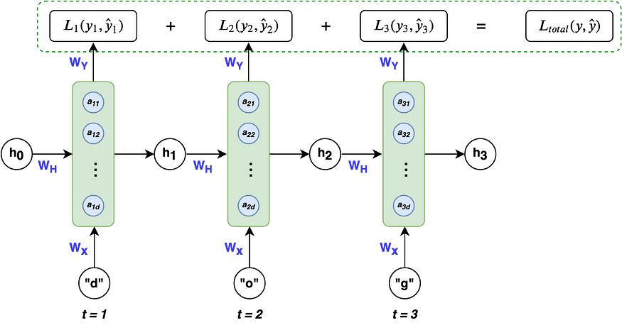
Because this example is a classification problem where we’re trying to predict four possible letters (“d-o-g-s”), it makes sense to use the multi-class cross entropy loss function:

Taking into account all time steps, the overall loss is:

Visually, this can be seen as:
Given our loss function, we need to calculate the gradients for our three weight matrices Wx, Wy, Wh, and update them with a learning rate η. Similar to normal backpropagation, the gradient gives us a sense of how the loss is changing with respect to each weight parameter. We update the weights to minimize loss with the following equation:

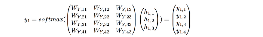
Now here comes the tricky part, calculating the gradient for Wx, Wy, and Wh. We’ll start by calculating the gradient for Wy because it’s the easiest. As stated before, the effect of the weights on loss spans over time. The weight gradient for Wy is the following:
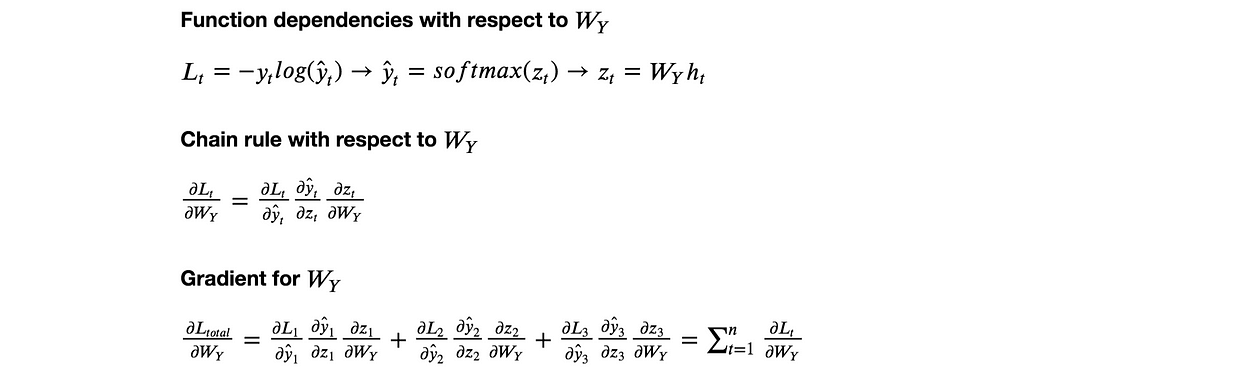
That’s the gradient calculation for Wy. Hopefully, pretty straight forward, the main idea is chain rule and to account for the loss at each time step.
The weight matrices Wx and Wh are analogous to each other, so we’ll just look at the gradient for Wx and leave Wh to you. One of the trickiest parts about calculating Wx is the recursive dependency on the previous state, as stated in line (2) in the image below. We need to account for the derivatives of the current error with respect to each of the previous states, which is done in (3). Finally, we again need to account for the loss at each time step (4).

And that’s backpropagation! Once we have the gradients for Wx, Wh, and Wy, we update them as usual and continue on with the backpropagation workflow. Now that you know how RNNs learn and make predictions, let’s go over one major flaw and then wrap up this post.
Note: See A Gentle Tutorial of Recurrent Neural Network with Error Backpropagation by Gang Chen² for a more detailed workflow on backpropagation through time with RNNs
One major problem: vanishing gradients
A problem that RNNs face, which is also common in other deep neural nets, is the vanishing gradient problem. Vanishing gradients make it difficult for the model to learn long-term dependencies. For example, if an RNN was given this sentence:

and had to predict the last two words “german” and “shepherd,” the RNN would need to take into account the inputs “brown”, “black”, and “dog,” which are the nouns and adjectives that describe a german shepherd. However, the word “brown” is quite far from the word “shepherd.” From the gradient calculation of Wx that we saw earlier, we can break down the backpropagation error of the word “shepherd” back to “brown” and see what it looks like:

The partial derivative of the state corresponding to the input “shepherd” respective to the state “brown” is actually a chain rule in itself, resulting in:

That’s a lot of chain rule! These chains of gradients are troublesome because if less than 1 they can cause the loss from the word shepherd with respect to the word brown to approach 0, thereby vanishing. This makes it difficult for the weights to take into account words that occur at the start of a long sequence. So the word “brown” when doing a forward propagation, may not have any effect in the prediction of “shepherd” because the weights weren’t updated due to the vanishing gradient. This is one of the major disadvantages of RNNs.
However, there have been advancements in RNNs such as gated recurrent units (GRUs) and long short term memory (LSTMs) that have been able to deal with the problem of vanishing gradients. We won’t cover them in this blog post, but in the future, I’ll be writing about GRUs and LSTMs and how they handle the vanishing gradient problem.
That’s it for this blog post. If you have any questions, comments, or feedback, feel free to comment down below. I hope you found this useful, thanks for reading!
References
[1]: Andrew Ng. Why Sequence Models. https://www.coursera.org/learn/nlp-sequence-models/lecture/0h7gT/why-sequence-models
[2]: Gang Chen. A Gentle Tutorial of Recurrent Neural Network with Error Backpropagation. https://arxiv.org/pdf/1610.02583.pdf
Join thousands of data leaders on the AI newsletter. Join over 80,000 subscribers and keep up to date with the latest developments in AI. From research to projects and ideas. If you are building an AI startup, an AI-related product, or a service, we invite you to consider becoming a sponsor.
Published via Towards AI
Towards AI Academy
We Build Enterprise-Grade AI. We'll Teach You to Master It Too.
15 engineers. 100,000+ students. Towards AI Academy teaches what actually survives production.
Start free — no commitment:
→ 6-Day Agentic AI Engineering Email Guide — one practical lesson per day
→ Agents Architecture Cheatsheet — 3 years of architecture decisions in 6 pages
Our courses:
→ AI Engineering Certification — 90+ lessons from project selection to deployed product. The most comprehensive practical LLM course out there.
→ Agent Engineering Course — Hands on with production agent architectures, memory, routing, and eval frameworks — built from real enterprise engagements.
→ AI for Work — Understand, evaluate, and apply AI for complex work tasks.
Note: Article content contains the views of the contributing authors and not Towards AI.
Related posts
Recent Posts
")


")


