


PyTorch LSTM — Shapes of Input, Hidden State, Cell State And Output
Last Updated on November 5, 2023 by Editorial Team
Author(s): Sujeeth Kumaravel
Originally published on Towards AI.
In Pytorch, to use an LSTM (with nn.LSTM()), we need to understand how the tensors representing the input time series, hidden state vector and cell state vector should be shaped. In this article, let us assume you are working with multivariate time series. Each multivariate time series in the dataset contains multiple univariate time series.
The following are the differences from pytorch’s LSTMCell discussed in the following link:
Pytorch LSTMCell — shapes of input, hidden state and cell state
In pytorch, to use an LSTMCell, we need to understand how the tensors representing the input time series, hidden state…
medium.com
- With nn.LSTM multiple layers of LSTM can be created by stacking them to form a stacked LSTM. The second LSTM takes the output of the first LSTM as input and so on.
2. dropout can be added in nn.LSTM class.
3. unbatched inputs can be given to nn.LSTM.
There is one more significant difference which will be discussed later in this post.
In this article we use the following terminology,
batch = number of multivariate time series in a single batch from the dataset
input_features = number of univariate time series in one multivariate time series
time steps = number of time steps in each multivariate time series
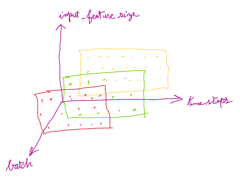
The batch of multivariate time series to be given as input to the LSTM should be a tensor of shape (time_steps, batch, input_features)
The following picture gives an understanding of this shape for input:
But, in LSTM, there is another way of shaping the input as well. This is explained below.
While initializing an LSTM object, the arguments input_features and hidden_size should be given.
Here,
input_features = number of univariate time series in one multivariate time series (same value as input_features mentioned above)
hidden_size = number of dimensions in the hidden state vector.
Other arguments that LSTM class can take:
num_layers = number of LSTM layers stacked on top of each other. When multiple layers are stacked on top of each other it is called a stacked LSTM. By default, the number of layer = 1
dropout = if non-zero, there will be a dropout layer added to the output of each LSTM layer with dropout probability equal this value. By default this value is 0 which means there is no dropout.
batch_first = if this is True, input and output tensors will have dimensions (batch, time_steps, input_features) instead of (time_steps, batch, input_features). By default, this is False.
proj_size = projection size. If proj_size > 0, LSTM with projections will be used.
The time series and the initial hidden state and the initial cell state should be given as input for a forward propagation through the LSTM.
The forward propagation of input, initial hidden state and initial cell state through the LSTM object should be in the format:
LSTM(input_time_series, (h_0, c_0))
Let’s see how to shape the hidden state vector and cell state vector before giving to LSTM for forward propagation.
h_0 — (num_layers, batch, h_out). Here h_out = proj_size if proj_size > 0 else hidden_size
c_0 — (num_layers, batch, hidden_size)
The following picture helps in understanding the hidden vectors shape.

A similar picture applies to cell state vectors also.
From the picture it can be understood that the dimensionality of the hidden and cell states for all layers is the same.
Consider the following code snippet:
import torch
import torch.nn as nn

lstm_0 = nn.LSTM(10, 20, 2) # (input_features, hidden_size, num_layers)
inp = torch.randn(4, 3, 10) # (time_steps, batch, input_features) -> input time series
h0 = torch.randn(2, 3, 20) # (num_layers, batch, hidden_size) -> initial value of hidden state
c0 = torch.randn(2, 3, 20) # (num_layers, batch, hidden_size) -> initial value of cell state

output, (hn, cn) = lstm_0(input, (h0, c0)) # forward pass of input through LSTM
Calling nn.LSTM() will call the __init__() dunder magic method and create the LSTM object. In the code above, this object is referenced as lstm_0.
In RNNs in general (LSTM is a type of RNN), each time_step of the input time series should be passed into the RNN one at a time in a sequence order to be processed by the RNN.
In order to process multivariate time series in a batch using an LSTM, each time_step in all MTSs in the batch should be passed through the LSTM sequentially.
A single call to the LSTM’s forward pass processes the entire series by processing each time step sequentially. This is different from LSTMCell in which a single call processes only one time_step and not the entire series.
The output of the code above is:
tensor([[[ 3.8995e-02, 1.1831e-01, 1.1922e-01, 1.3734e-01, 1.6157e-02,
 3.3094e-02, 2.8738e-01, -6.9250e-02, -1.8313e-01, -1.2594e-01,
 1.4951e-01, -3.2489e-01, 2.1723e-01, -1.1722e-01, -2.5523e-01,
 -6.5740e-02, -5.2556e-02, -2.7092e-01, 3.0432e-01, 1.4228e-01],
 [ 9.2476e-02, 1.1557e-02, -9.3600e-03, -5.2662e-02, 5.5299e-03,
 -6.2017e-02, -1.9826e-01, -2.7072e-01, -5.5575e-02, -2.3024e-03,
 -2.6832e-01, -5.8481e-01, -8.3415e-03, -2.8817e-01, 4.6101e-03,
 3.5043e-02, -6.2501e-01, 4.2930e-02, -5.4698e-01, -5.8626e-01],
 [-2.8034e-01, -3.4194e-01, -2.1888e-02, -2.1787e-01, -4.0497e-01,
 -3.6124e-01, -1.5303e-01, -1.3310e-01, -3.7745e-01, -1.8368e-01,
 -2.7527e-01, -2.5508e-01, 4.0958e-01, 9.0280e-02, 3.0029e-02,
 -3.0227e-01, -8.7728e-02, 2.9999e-01, 1.1918e-01, -3.5911e-01]],

 [[ 3.3873e-02, 2.9018e-04, 1.5477e-01, -6.2761e-02, 1.5835e-02,
 3.6805e-03, 2.2269e-01, -5.5305e-03, -1.2751e-01, -4.8088e-02,
 1.2078e-01, -2.8451e-01, 1.5305e-01, -1.3836e-01, -1.0816e-01,
 -4.0884e-02, 2.6503e-03, -2.2445e-01, 2.4591e-01, -3.3629e-02],
 [ 4.3514e-02, -1.7708e-02, 3.2486e-02, -2.9323e-02, -6.9395e-02,
 -1.7256e-01, -1.2758e-01, -1.2148e-01, -6.5050e-02, 8.1324e-02,
 -2.6087e-01, -2.8995e-01, 9.4633e-02, -3.3044e-01, 4.1104e-02,
 3.1116e-02, -2.0361e-01, 4.9253e-02, -1.2465e-01, -3.5137e-01],
 [-2.3935e-01, -1.8981e-01, 6.8023e-04, -1.0812e-01, -3.0005e-01,
 -2.5705e-01, -8.1085e-03, -7.1204e-02, -2.1569e-01, -5.1020e-02,
 -1.2772e-01, -2.0699e-01, 2.5266e-01, 2.8209e-02, 1.2555e-01,
 -6.3178e-02, -6.0789e-02, 1.7691e-01, 1.5729e-01, -2.9594e-01]],

 [[ 2.5303e-02, -6.8317e-02, 7.2816e-02, -8.7644e-02, 1.7320e-02,
 4.5144e-03, 1.6791e-01, 3.3909e-02, -8.8614e-02, 1.0397e-02,
 4.9521e-02, -2.3401e-01, 1.2013e-01, -1.3862e-01, -5.1140e-02,
 4.5510e-03, 3.9663e-02, -1.7712e-01, 2.2307e-01, -1.1596e-01],
 [ 1.7504e-02, -6.9332e-02, 1.9985e-02, -6.1289e-02, -7.1808e-02,
 -1.3141e-01, -2.9575e-02, -5.4011e-02, -9.2560e-02, 7.3578e-02,
 -1.8498e-01, -2.2349e-01, 1.1977e-01, -2.3788e-01, 5.5626e-02,
 4.7339e-02, -2.8371e-02, 3.9558e-02, 5.2823e-02, -3.2909e-01],
 [-1.1658e-01, -1.4822e-01, -1.2125e-03, -6.8908e-02, -1.9544e-01,
 -1.4223e-01, 6.0825e-02, -1.9438e-02, -1.7269e-01, -1.3336e-02,
 -8.5011e-02, -2.0159e-01, 1.6916e-01, -2.8147e-02, 1.3812e-01,
 -3.0235e-03, 2.6134e-02, 9.0310e-02, 1.6692e-01, -2.6583e-01]],

 [[ 2.7330e-02, -1.0817e-01, 2.4307e-02, -9.2434e-02, 7.7234e-03,
 3.5870e-02, 1.2094e-01, 5.4508e-02, -8.3826e-02, 1.3931e-02,
 8.6096e-03, -2.1100e-01, 8.7992e-02, -1.3711e-01, -1.7072e-02,
 3.3240e-02, 5.0868e-02, -1.4814e-01, 2.0445e-01, -1.7466e-01],
 [ 8.6976e-03, -9.4327e-02, 1.1120e-02, -6.1805e-02, -3.7574e-02,
 -1.2975e-01, 4.9702e-02, 7.1489e-03, -9.0461e-02, 6.9983e-02,
 -1.2824e-01, -2.1042e-01, 1.3504e-01, -1.6717e-01, 6.9663e-02,
 6.7910e-02, 5.1151e-02, 1.8291e-02, 1.5308e-01, -2.6023e-01],
 [-7.0474e-02, -1.2629e-01, 9.9434e-03, -7.9685e-02, -1.0742e-01,
 -7.5179e-02, 1.0198e-01, 2.5444e-02, -1.3823e-01, -6.7337e-04,
 -7.8697e-02, -1.9341e-01, 1.2829e-01, -7.2150e-02, 1.1318e-01,
 2.5169e-02, 7.6451e-02, 2.3822e-02, 1.8464e-01, -2.3790e-01]]],
 grad_fn=<MkldnnRnnLayerBackward0>)
In this output there are 4 arrays corresponding to the 4 time steps. Each of these time_steps contains 3 arrays corresponding to the 3 MTS in the batch. Each of these 3 arrays contains 20 elements -> this is the hidden state. Hence for each x_t vector in each time_step in each MTS, a hidden state is output. These are the hidden states in the last layer of the stacked LSTM.
Output: (output_multivariate_time_series, (h_n, c_n))
If you print hn which is present in the code above, the following is the output:
tensor([[[-0.3046, -0.1601, -0.0024, -0.0138, -0.1810, -0.1406, -0.1181,
 0.0634, 0.0936, -0.1094, -0.2822, -0.2263, -0.1090, 0.2933,
 0.0760, -0.1877, -0.0877, -0.0813, 0.0848, 0.0121],
 [ 0.0349, -0.2068, 0.1353, 0.1121, 0.1940, -0.0663, -0.0031,
 -0.2047, -0.0008, -0.0439, -0.0249, 0.0679, -0.0530, 0.1078,
 -0.0631, 0.0430, 0.0873, -0.1087, 0.3161, -0.1618],
 [-0.0528, -0.2693, 0.1001, -0.1097, 0.0097, -0.0677, -0.0048,
 0.0509, 0.0655, 0.0075, -0.1127, -0.0641, 0.0050, 0.1991,
 0.0370, -0.0923, 0.0629, 0.0122, 0.0688, -0.2374]],

 [[ 0.0273, -0.1082, 0.0243, -0.0924, 0.0077, 0.0359, 0.1209,
 0.0545, -0.0838, 0.0139, 0.0086, -0.2110, 0.0880, -0.1371,
 -0.0171, 0.0332, 0.0509, -0.1481, 0.2044, -0.1747],
 [ 0.0087, -0.0943, 0.0111, -0.0618, -0.0376, -0.1297, 0.0497,
 0.0071, -0.0905, 0.0700, -0.1282, -0.2104, 0.1350, -0.1672,
 0.0697, 0.0679, 0.0512, 0.0183, 0.1531, -0.2602],
 [-0.0705, -0.1263, 0.0099, -0.0797, -0.1074, -0.0752, 0.1020,
 0.0254, -0.1382, -0.0007, -0.0787, -0.1934, 0.1283, -0.0721,
 0.1132, 0.0252, 0.0765, 0.0238, 0.1846, -0.2379]]],
 grad_fn=<StackBackward0>)
This contains the hidden state vectors in the first layer and the second layer in the stacked LSTM for the last time_step in each of the 3 MTS in the batch. If you notice, the second layer (last layer) hidden state is the same as the last time step hidden state in the output mentioned previously.
So, the output MTS dimensionality is (time_steps, batch, hidden_size).
This output dimensionality can be understood from the picture below:

h_n dimensionality: (num_layers, batch, h_out)
c_n dimensionality: (num_layers, batch, hidden_size)
Join thousands of data leaders on the AI newsletter. Join over 80,000 subscribers and keep up to date with the latest developments in AI. From research to projects and ideas. If you are building an AI startup, an AI-related product, or a service, we invite you to consider becoming a sponsor.
Published via Towards AI
Related posts


Popular posts

 for 2021")


Updates

Recent Posts


