Perceptron Is Not SGD: A Better Interpretation Through Pseudogradients

Last Updated on October 29, 2021 by Editorial Team

Author(s): Francesco Orabona, Ph.D.

Perceptron Is Not SGD: A Better Interpretation Through Pseudogradients — Actual conversation with my wife (Image from xkcd.com)

There is a popular interpretation of the Perceptron as a stochastic (sub)gradient descent procedure. I even found slides online with this idea. The thought of so many young minds twisted by these false claims was too much to bear. So, I felt compelled to write a blog post to explain why this is wrong… 😉
Moreover, I will also give a different and (I think) much better interpretation of the Perceptron algorithm.

1. Perceptron Algorithm

The Perceptron algorithm was introduced by Rosenblatt in 1958. To be more precise, he introduced a family of algorithms characterized by a certain architecture. Also, he considered what we call now supervised and unsupervised training procedures. However, nowadays when we talk about the Perceptron we intend the following algorithm:

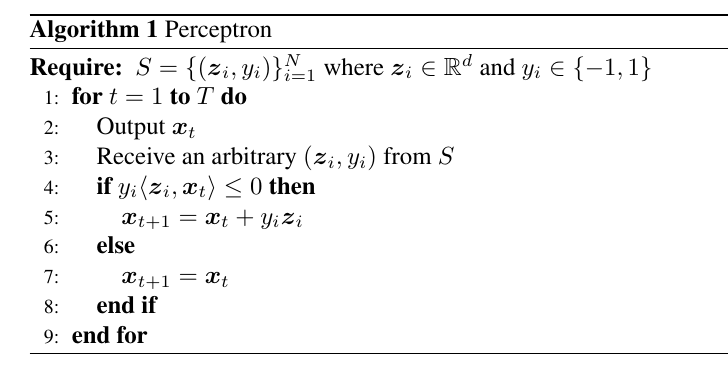
In the algorithm, the couples ${({\boldsymbol z}_t,y_t)}$ for ${t=1,\dots,N}$ , with ${{\boldsymbol x}_t \in {\mathbb R}^d}$ and ${y_t \in \{-1, 1\}}$ , represent a set of ${N}$ input/output pairs that we want to learn to classify correctly in the two categories ${+1}$ and ${-1}$ . We assume that there exists an unknown vector ${{\boldsymbol u}}$ the correctly classify all the samples, that is ${\rm sign(\langle {\boldsymbol z}_t, {\boldsymbol u}\rangle) = y_t}$ . Note that any scaling of ${{\boldsymbol u}}$ by a positive constant still correctly classify all the samples, so there are infinite solutions. The aim of the Perceptron is to find any of these solutions.

From an optimization point of view, this is called a feasibility problem, that is something like

$\displaystyle \begin{aligned} Find & \ {\boldsymbol x} \\ s.t. & \ {\boldsymbol x} \in C, \end{aligned}$

where ${C}$ is some set. They are an essential step in constrained optimization for algorithms that require an feasible initial point. Feasibility problems are not optimization problems even if in some cases can be solved with an optimization formulation.

In the Perceptron case, we can restate the problem as

$\displaystyle \begin{aligned} Find & \ {\boldsymbol x}\\ s.t. & \ y_i \langle {\boldsymbol z}_i,{\boldsymbol x}\rangle \geq 1 , i=1, \dots, N, \end{aligned}$

where the “1” on the r.h.s. is clearly arbitrary and it can be changed through rescaling of ${{\boldsymbol x}}$ . So, in optimization language, the Perceptron algorithm is nothing else than an iterative procedure to solve the above feasibility problem.

2. Issues with the SGD Interpretation

As said above, sometimes people refer to the Perceptron as a stochastic (sub)gradient descent algorithm on the objective function

$\displaystyle \label{eq:obj_relu_perceptron} F({\boldsymbol x}) = \sum_{i=1}^N \max(-y_i \langle {\boldsymbol z}_i,{\boldsymbol x}\rangle,0)~. \ \ \ \ \ (1)$

I think they are many problems with this ideas, let me list some of them

First of all, the above interpretation assumes that we take the samples randomly from ${S}$ . However, this is not needed in the Perceptron and it was not needed in the first proofs of the Perceptron convergence (Novikoff, 1963). There is a tendency to call anything that receive one sample at a time as “stochastic”, but “arbitrary order” and “stochastic” are clearly not the same.
The Perceptron is typically initialized with ${{\boldsymbol x}_1=\boldsymbol{0}}$ . Now, we have two problems. The first one is that with a black-box first-order oracle, we would get a subgradient of a ${\max(-y_i \langle {\boldsymbol z}_i,{\boldsymbol x}\rangle,0)}$ , where ${i}$ is drawn uniformly at random in ${[1,N]}$ . A possible subgradient for any ${i}$ is ${\boldsymbol{0}}$ . This means that SGD would not update. Instead, the Perceptron in this case does update. So, we are forced to consider a different model than the black-box one. Changing the oracle model is a minor problem, but this fact hints to another very big issue.
The biggest issue is that ${{\boldsymbol x}_1=\boldsymbol{0}}$ is a global optimum of ${F}$ ! So, there is nothing to minimize, we are already done in the first iteration. However, from a classification point of view, this solution seems clearly wrong. So, it seems we constructed an objective function we want to minimize and a corresponding algorithm, but for some reason we do not like one of its infinite minimizers. So, maybe, the objective function is wrong? So, maybe, this interpretation misses something?

There is an easy way to avoid some of the above problems: change the objective function to a parametrized loss that has non-zero gradient in zero. For example, something like this

$\displaystyle F_\alpha({\boldsymbol x}) = \sum_{i=1}^N \log(1+\exp(-\alpha y_i \langle {\boldsymbol z}_i,{\boldsymbol x}\rangle))~.$

Now, when ${\alpha}$ goes to infinity, you recover the function ${F}$ . However, for any finite ${\alpha}$ , ${\boldsymbol{0}}$ is not a global optimum anymore. As a side effect, we also solved the issue of the subgradient of the max function. In this way, you could interpret the Perceptron algorithm as the limit behaviour of SGD on a family of optimization problems.

To be honest, I am not sure this is a satisfying solution. Moreover, the stochasticity is still there and it should be removed.

Now, I already proved a mistake bound for the Perceptron, without any particular interpretation attached to it. As a matter of fact, proofs do not need interpretations to be correct. I showed that the Perceptron competes with a family of loss functions that implies that it does not just use the subgradient of a single function. However, if you need an intuitive way to think about it, let me present you the idea of pseudogradients.

3. Pseudogradients

Suppose we want to minimize a function ${L}$ -smooth ${F}$ and we would like to use something like gradient descent. However, we do not have access to its gradient. In this situation, (Polyak and Tsypkin, 1973) proposed to use a “pseudogradient”, that is any vector ${{\boldsymbol g}}$ that forms an angle of 90 degrees or less with the actual gradient in ${{\boldsymbol x}}$

$\displaystyle \langle {\boldsymbol g}, \nabla F({\boldsymbol x})\rangle \geq \gamma \geq 0~.$

In a very intuitive way, ${{\boldsymbol g}}$ gives me some information that should allow me to minimize ${F}$ , at least in the limit. The algorithm then becomes a “pseudogradient descent” procedure that updates the current solution in the direction of the negative pseudogradient

$\displaystyle {\boldsymbol x}_{t+1} = {\boldsymbol x}_t - \eta_t {\boldsymbol g}_t,$

where ${\eta_t\geq0}$ are the step size or learning rates.

Note that (Polyak and Tsypkin, 1973) define the pseudogradients as a stochastic vector that satisfies the above inequality in conditional expectation and for a time-varying ${\gamma}$ . Indeed, there are a number of very interesting results in that paper. However, for simplicity of exposition I will only consider the deterministic case and only describe the application to the Perceptron.

Let’s see how this would work. Let’s assume that ${\gamma>0}$ at least for an initial number of rounds, that means that the angle between the pseudogradient and the gradient is acute. From the ${L}$ -smoothness of ${F}$ , we have that

$\displaystyle \begin{aligned} F({\boldsymbol x}_{t+1}) &\leq F({\boldsymbol x}_t) +\langle \nabla F({\boldsymbol x}_t), {\boldsymbol x}_{t+1} - {\boldsymbol x}_t\rangle + \frac{L}{2}\|{\boldsymbol x}_{t+1}-{\boldsymbol x}_t\|^2 \\ &= F({\boldsymbol x}_t) - \eta_t \langle \nabla F({\boldsymbol x}_t), {\boldsymbol g}_t \rangle + \eta_t^2 \frac{L}{2}\|{\boldsymbol g}_t\|^2 \\ &\leq F({\boldsymbol x}_t) - \eta_t \gamma + \eta_t^2 \frac{L}{2}\|{\boldsymbol g}_t\|^2~. \end{aligned}$

Now, if ${0 < \eta_t < \frac{2\gamma}{L \|{\boldsymbol g}\|^2}}$ , we have that ${- \eta_t \gamma + \eta_t^2 \frac{L}{2}\|{\boldsymbol g}_t\|^2<0}$ so can guarantee that the value of ${F}$ decreases at each step. So, we are minimizing ${F}$ without using a gradient!

To get a rate of convergence, we should know something more about ${{\boldsymbol g}_t}$ . For example, we could assume that ${\|{\boldsymbol g}_t\|\leq G}$ . Then, setting ${\eta_t = \frac{\gamma^2}{L G^2}}$ , we obtain

$\displaystyle F({\boldsymbol x}_{t+1}) \leq F({\boldsymbol x}_t) - \frac{\gamma^2}{2 L G^2}~.$

This is still not enough because it is clear that ${\gamma>0}$ cannot be true on all rounds because when we are in the minimizer ${\nabla F({\boldsymbol x}_t)=\boldsymbol{0}}$ . However, with enough assumptions, following this route you can even get a rate of convergence.

4. Pseudogradients for the Perceptron

How do we use this to explain the Perceptron? Suppose your set ${S}$ is linearly separable with a margin of 1. This means that there exists a vector ${{\boldsymbol u}\in {\mathbb R}^d}$ such that

$\displaystyle \label{eq:margin_assumption} \min_i y_i \langle {\boldsymbol z}_i, {\boldsymbol u}\rangle = 1~. \ \ \ \ \ (2)$

Note that the value of the margin is arbitrary, we can change it just rescaling ${{\boldsymbol u}}$ .

Remark 1. An equivalent way to restate this condition is to constrain ${{\boldsymbol u}}$ to have unitary norm and require

$\displaystyle \min_i y_i \langle {\boldsymbol z}_i, {\boldsymbol u}\rangle = \gamma,$

where ${\gamma>0}$ is called the maximum margin of ${S}$ . However, in the following I will not use the margin notation because it makes things a bit less clear from an optimization point of view.

We would like to construct an algorithm to find ${{\boldsymbol u}}$ (or any positive scaling of it) from the samples ${\{({\boldsymbol z}_i,y_i)\}_{i=1}^N}$ . So, we need an objective function. Here the brilliant idea of Polyak and Tsypkin: in each iteration take an arbitrary ${({\boldsymbol z}_i,y_i)}$ and define ${{\boldsymbol g}_t = -y_i {\boldsymbol z}_i \boldsymbol{1}[y_i \langle {\boldsymbol z}_i, {\boldsymbol x}_t\rangle \leq 0]}$ , that is exactly the negative update we use in the Perceptron. This turns out to be a pseudogradient for ${F({\boldsymbol x}) = \frac{1}{2}\|{\boldsymbol x}-{\boldsymbol u}\|^2}$ . Indeed,

$\displaystyle \begin{aligned} \langle {\boldsymbol g}_t, \nabla F({\boldsymbol x}_t) \rangle &= \langle -y_i {\boldsymbol z}_i \boldsymbol{1}[y_i \langle {\boldsymbol z}_i, {\boldsymbol x}_t\rangle \leq 0], {\boldsymbol x}_t-{\boldsymbol u}\rangle \\ &= \boldsymbol{1}[y_i \langle {\boldsymbol z}_i, {\boldsymbol x}_t\rangle \leq 0](\langle -y_i {\boldsymbol z}_i, {\boldsymbol x}_t\rangle + y_i \langle {\boldsymbol z}_i, {\boldsymbol u}\rangle) \\ &\geq \boldsymbol{1}[y_i \langle {\boldsymbol z}_i, {\boldsymbol x}_t\rangle \leq 0], \end{aligned}$

where in the last inequality we used (2).

Let’s pause for a moment to look at what we did: We want to minimize ${F({\boldsymbol x})=\frac{1}{2}\|{\boldsymbol x}-{\boldsymbol u}\|^2}$ , but its gradient is just impossible to calculate because it depends on ${{\boldsymbol u}}$ that we clearly do not know. However, every time the Perceptron finds a sample on which its prediction is wrong, we can construct a pseudogradient, without any knowledge of ${{\boldsymbol u}}$ . It is even more surprising if you consider the fact that there is an infinite number of possible solutions ${{\boldsymbol u}}$ and hence functions ${F}$ , yet the pseudogradient correlates positively with the gradient of any of them! Moreover, no stochasticity is necessary.

At this point we are basically done. In fact, observe that ${F({\boldsymbol x}) =\frac{1}{2}\|{\boldsymbol x}-{\boldsymbol u}\|^2}$ is 1-smooth. So, every time ${{\boldsymbol g}_t\neq \boldsymbol{0}}$ , the analysis above tells us that

$\displaystyle \begin{aligned} \frac{1}{2}\|{\boldsymbol x}_{t+1}-{\boldsymbol u}\|^2 - \frac{1}{2}\|{\boldsymbol x}_t - {\boldsymbol u}\|^2 \leq -\eta_t + \frac{\eta_t^2}{2} \|{\boldsymbol z}_t\|^2 \leq -\eta_t + \frac{\eta_t^2}{2} G^2, \end{aligned}$

where in the last inequality we have assumed ${\|{\boldsymbol z}_t\|\leq G}$ .

Setting ${\eta_t=\eta}$ , summing over time, and denoting ${M}$ the number of updates we have over ${T}$ iterations, we obtain

$\displaystyle M \leq \frac{\eta M G^2}{2} + \frac{1}{2\eta}\|{\boldsymbol u}-{\boldsymbol x}_1\|^2 - \frac{1}{2\eta} \|{\boldsymbol u}-{\boldsymbol x}_{T+1}\|^2 \leq \frac{\eta M G^2}{2} + \frac{1}{2\eta}\|{\boldsymbol u}\|^2,$

where used the fact that ${{\boldsymbol x}_1=\boldsymbol{0}}$ .

Now, there is the actual magic of the (parameter-free!) Perceptron update rule: as we explained here, the updates of the Perceptron are independent of ${\eta>0}$ . That is, given an order in which the samples are presented to the algorithm, any fixed ${\eta}$ makes the Perceptron update on the same samples and it only changes the scale of ${{\boldsymbol x}_t}$ . Hence, even if the Perceptron algorithm uses ${\eta=1}$ , we can consider an arbitrary ${\eta}$ decided post-hoc to minimize the upper bound. Hence, we obtain

$\displaystyle M \leq G \|{\boldsymbol u}\|\sqrt{M},$

that is

$\displaystyle M \leq G^2 \|{\boldsymbol u}\|^2~.$

Now, observing that the r.h.s. is independent of ${T}$ , we proved that the maximum number of updates, or equivalently mistakes, of the Perceptron algorithm is bounded.

Are we done? Not yet! We can now improve the Perceptron algorithm taking full advantage of the pseudogradients interpretation.

5. An Improved Perceptron

This is a little known idea to improve the Perceptron. It can be shown with the classic analysis as well, but it comes very naturally from the pseudogradient analysis.

Let’s start from

$\displaystyle \frac{1}{2}\|{\boldsymbol x}_{t+1}-{\boldsymbol u}\|^2 - \frac{1}{2}\|{\boldsymbol x}_t - {\boldsymbol u}\|^2 \leq -\eta_t + \frac{\eta_t^2}{2} \|{\boldsymbol z}_t\|^2~.$

Now consider only the rounds in which ${{\boldsymbol z}_t\neq \boldsymbol{0}}$ and set ${\eta_t = \frac{1}{\|{\boldsymbol z}_t\|^2}}$ , that is obtained by an optimization of the expression ${-\eta_t + \frac{\eta_t^2}{2} \|{\boldsymbol z}_t\|^2}$ . So, we obtain

$\displaystyle \label{eq:improved_perc_1} \frac{1}{2}\|{\boldsymbol x}_{t+1}-{\boldsymbol u}\|^2 - \frac{1}{2}\|{\boldsymbol x}_t - {\boldsymbol u}\|^2 \leq -\frac{1}{2\|{\boldsymbol z}_t\|^2}~. \ \ \ \ \ (3)$

This means that now the update rule becomes

$\displaystyle {\boldsymbol x}_{t+1} = {\boldsymbol x}_t + \frac{y_i {\boldsymbol z}_i}{\|{\boldsymbol z}_i\|^2} \boldsymbol{1}[y_i \langle {\boldsymbol z}_i, {\boldsymbol x}_t \rangle \leq 0]~.$

Now, summing (3) over time, we get

$\displaystyle \sum_{i=1}^M \frac{1}{\|{\boldsymbol z}_i\|^2} \leq \|{\boldsymbol u}\|^2 - \|{\boldsymbol x}_{T+1}-{\boldsymbol u}\|^2 \leq \|{\boldsymbol u}\|^2~.$

It is clear that this inequality implies the previous one because ${\sum_{i=1}^M \frac{1}{\|{\boldsymbol z}_i\|^2} \geq \frac{M}{G^2}}$ . But we can even obtain a tighter bound. Using the inequality between harmonic, geometric, and arithmetic mean, we have

$\displaystyle M \leq \|{\boldsymbol u}\|^2 \frac{M}{\sum_{i=1}^M \frac{1}{\|{\boldsymbol z}_i\|^2}} \leq \|{\boldsymbol u}\|^2 \left(\prod_{i=1}^M \|{\boldsymbol z}_i\|^2\right)^{1/M} \leq \|{\boldsymbol u}\|^2 \frac{1}{M} \sum_{i=1}^M \|{\boldsymbol z}_i\|^2 \leq \|{\boldsymbol u}\|^2 G^2~.$

In words, the original Perceptron bound depends on the maximum squared norm of the samples on which we updated. Instead, this bound depends on the geometric or arithmetic mean of the squared norm of the samples on which we updated, that is less or equal to the maximum.

6. Pseudogradients and Lyapunov Potential Functions

Some people might have realized yet another way to look at this: ${F({\boldsymbol x}) = \frac{1}{2}\|{\boldsymbol x}-{\boldsymbol u}\|^2}$ is the Lyapunov function typically used to analyze subgradient descent. In fact, the classic analysis of SGD considers the guaranteed decrement at each step of this function. The two things coincide, but I find the pseudogradient idea to add a non-trivial amount of information because it allows to bypass the idea of using a subgradient of the loss function completely.

Moreover, the idea of the pseudogradients is more general because it applies to any smooth function, not only to the choice of ${F({\boldsymbol x}) = \frac{1}{2}\|{\boldsymbol x}-{\boldsymbol u}\|^2}$ .

Overall, it is clear that all the good analyses of the Perceptron must have something in common. However, sometimes recasting a problem in a particular framework might have some advantages because it helps our intuition. In this view, I find the pseudogradient view particularly compelling because it aligns with my intuition of how an optimization algorithm is supposed to work.

7. History Bits

I already wrote about the Perceptron, so I will just add few more relevant bits.

As I said, it seems that the family of Perceptrons algorithms was intended to be something much more general than what we intend now. The particular class of Perceptron we use nowadays was called ${\alpha}$ -system (Block, 1962). I hypothesize that the fact the ${\alpha}$ -system survived the test of time is exactly due to the simple convergence proof in (Block, 1962) and (Novikoff, 1963). Both proofs are non-stochastic. For the sake of proper credits assignment, it seems that the convergence proof of the Perceptron was proved by many others before Block and Novikoff (see references in Novikoff, 1963). However, the proof in (Novikoff, 1963) seems to be the cleanest one. (Aizerman, Braverrnan, and Rozonoer, 1964) (essentially) describe for the first time the Kernel Perceptron and prove a finite mistake bound for it.

I got the idea of smoothing the Perceptron algorithm with a scaled logistic loss from a discussion on Twitter with Maxim Raginsky. He wrote that (Aizerman, Braverrnan, and Rozonoer, 1970) proposed some kind of smoothing in a Russian book for the objective function in (1), but I don’t have access to it so I am not sure what are the details. I just thought of a very natural one.

The idea of pseudogradients and the application to the Perceptron algorithm is in (Polyak and Tsypkin, 1973). However, there the input/output samples are still stochastic and the finite bound is not explicitly calculated. As I have shown, stochasticity is not needed. It is important to remember that online convex optimization as a field will come much later, so there was no reason for these people to consider arbitrary or even adversarial order of the samples.

The improved Perceptron mistake bound could be new (but please let me know if it isn’t!) and it is inspired from the idea in (Graepel, Herbrich, and Williamson, 2001) of normalizing the samples to show a tighter bound.

Acknowledgements

Given the insane amount of mistakes that Nicolò Campolongo usually finds in my posts, this time I asked him to proofread it. So, I thank Nicolò for finding an insane amount of mistakes on a draft of this post 🙂

Bio: Francesco Orabona is an Assistant Professor at Boston University. He received his Ph.D. in Electronic Engineering from the University of Genoa, Italy, in 2007. As a result of his activities, Dr. Orabona has published more than 70 papers in scientific journals and conferences on the topics of online learning, optimization, and statistical learning theory. His latest work is on “parameter-free” machine learning and optimization algorithms, that is algorithms that achieve the best performance without the need to tune parameters, like regularization, learning rate, momentum, etc.

Perceptron Is Not SGD: A Better Interpretation Through Pseudogradients was originally published in Parameter-Free Learning and Optimization Algorithms, where people are continuing the conversation by highlighting and responding to this story.

Published via Towards AI

Frequently Used, Contextual References

Resources

Publication

Perceptron Is Not SGD: A Better Interpretation Through Pseudogradients

Author(s): Francesco Orabona, Ph.D.

Towards AI Team

Feedback ↓ Cancel reply

Popular posts

Best Laptops for Deep Learning, Machine Learning (ML), and Data Science for 2023

Best Workstations for Deep Learning, Data Science, and Machine Learning (ML) for 2022

Descriptive Statistics for Data-driven Decision Making with Python

Best Machine Learning (ML) Books - Free and Paid - Editorial Recommendations for 2022

Best Data Science Books - Free and Paid - Editorial Recommendations for 2022

Updates

Recent Posts

Learn AI Together — Towards AI Community Newsletter #21

Top Important LLM Papers for the Week from 15/04 to 21/04

Meta LLAMA 3 — Most Capable Open LLM

Introduction of Neural Style Transfer – A Pioneer in Generative AI

Top Important Computer Vision Papers for the Week from 15/04 to 21/04

The World’s Leading AI and Technology Publication.

Company

CONTACT US

Cookie	Duration	Description
cookielawinfo-checkbox-analytics	11 months	This cookie is set by GDPR Cookie Consent plugin. The cookie is used to store the user consent for the cookies in the category "Analytics".
cookielawinfo-checkbox-functional	11 months	The cookie is set by GDPR cookie consent to record the user consent for the cookies in the category "Functional".
cookielawinfo-checkbox-necessary	11 months	This cookie is set by GDPR Cookie Consent plugin. The cookies is used to store the user consent for the cookies in the category "Necessary".
cookielawinfo-checkbox-others	11 months	This cookie is set by GDPR Cookie Consent plugin. The cookie is used to store the user consent for the cookies in the category "Other.
cookielawinfo-checkbox-performance	11 months	This cookie is set by GDPR Cookie Consent plugin. The cookie is used to store the user consent for the cookies in the category "Performance".
viewed_cookie_policy	11 months	The cookie is set by the GDPR Cookie Consent plugin and is used to store whether or not user has consented to the use of cookies. It does not store any personal data.

Frequently Used, Contextual References

Resources

Publication

Perceptron Is Not SGD: A Better Interpretation Through Pseudogradients

Author(s): Francesco Orabona, Ph.D.

Towards AI Team

Related posts

Feedback ↓ Cancel reply

Popular posts

Updates

Recent Posts

The World’s Leading AI and Technology Publication.

Company

CONTACT US

GDPR CCPA Statement