House Price Predictions Using Keras

Last Updated on February 25, 2021 by Editorial Team

Author(s): PRATIYUSH MISHRA

Deep Learning

Implementing neural networks using Keras along with hyperparameter tuning to predict house prices.

This is a starter tutorial on modeling using Keras which includes hyper-parameter tuning along with callbacks.

Problem Statement

Creating a Keras-Regression model that can accurately analyse features of a given house and predict the price accordingly.

Steps Involved

1. Analysis and Imputation of missing values
2. One-Hot Encoding of Categorical Features
3. Exploratory Data Analysis(EDA) & Outliers Detection.
4. Keras-Regression Modelling along with hyper-parameter tuning.
5. Training the Model along with EarlyStopping Callback.
6. Prediction and Evaluation

Kaggle Notebook Link

Importing Libraries

We would be using numpy and pandas for processing our dataset, matplotlib and seaborn for data visualization, and Keras for implementing our neural network. Also, we would be using Sklearn for outlier detection and scaling our dataset.

import numpy as np
import pandas as pd
import matplotlib.pyplot as plt
import seaborn as sns
sns.set()
from sklearn.preprocessing import StandardScaler # Standardization
from sklearn.ensemble import IsolationForest # Outlier Detection
from keras.models import Sequential # Sequential Neural Network
from keras.layers import Dense
from keras.callbacks import EarlyStopping # Early Stopping Callback
from keras.optimizers import Adam # Optimizer
from kerastuner.tuners import RandomSearch # HyperParameter Tuning
import warnings
warnings.filterwarnings('ignore') # To ignore warnings.

Loading the Dataset

Here we have used the Dataset from House Prices — Advanced Regression Techniques

train = pd.read_csv('../input/house-prices-advanced-regression-techniques/train.csv')
test = pd.read_csv('../input/house-prices-advanced-regression-techniques/test.csv')
y = train['SalePrice'].values
data = pd.concat([train,test],axis=0,sort=False)
data.drop(['SalePrice'],axis=1,inplace=True)
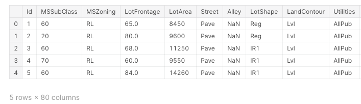
data.head()

Analysis and Imputation of missing values

We would first see all the features having missing values. This would include data from both training and testing data.

missing_values = data.isnull().sum()
missing_values = missing_values[missing_values > 0].sort_values(ascending = False)
NAN_col = list(missing_values.to_dict().keys())
missing_values_data = pd.DataFrame(missing_values)
missing_values_data.reset_index(level=0, inplace=True)
missing_values_data.columns = ['Feature','Number of Missing Values']
missing_values_data['Percentage of Missing Values'] = (100.0*missing_values_data['Number of Missing Values'])/len(data)
missing_values_data

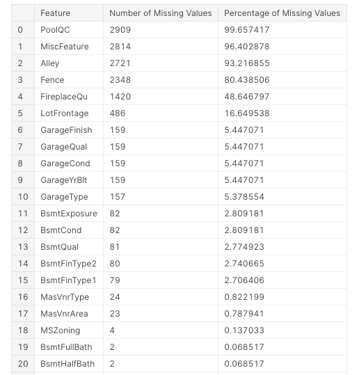
There are in total 33 features having missing values. Although in some of the top features in terms of percentage of missing values such as PoolQC, the missing value is representing that the house simply does not have that feature(in this case house does not have a pool) which is evident from the Pool Area feature which shows a value of 0 corresponding to all the missing values of PoolQC feature. We fill the missing values in the following way:

• Basement: This includes BsmtFinSF1, BsmtFinSF2, TotalBsmtSF and BsmtUnfSF. We would fill all missing values with 0 since the NAN values here simply represent that the house does not have a basement so the area of the basement would be 0.
• Electrical: Only one row has a missing value for this feature. Therefore after manual inspection, we would put its value to be ‘FuseA’
• KitchenQual: Again since only one row has a missing value for this, therefore we put ‘TA’ for this which is the most common value for this feature in the dataset.
• LotFrontage: Here we would first fill all missing values by taking the mean of the LotFrontage values of all groups having the same values of 1stFlrSF. This is because LotFrontage has a high correlation with 1stFlrSF. However, there can be cases where all the LotFrontage values corresponding to a particular 1stFlrSF value can be missing. To tackle such cases we would then fill it by using interpolate function of pandas to fill missing values linearly.
• MasVnrArea: Again we would be applying the same analogy as we did above with LotFrontage.
• Others: For other features, we would follow the most generic approach, that is, we would fill numeric ones by the mean of all the values of that feature and for categorical we would fill it by NA.

data['BsmtFinSF1'].fillna(0, inplace=True)
data['BsmtFinSF2'].fillna(0, inplace=True)
data['TotalBsmtSF'].fillna(0, inplace=True)
data['BsmtUnfSF'].fillna(0, inplace=True)
data['Electrical'].fillna('FuseA',inplace = True)
data['KitchenQual'].fillna('TA',inplace=True)
data['LotFrontage'].fillna(data.groupby('1stFlrSF')['LotFrontage'].transform('mean'),inplace=True)
data['LotFrontage'].interpolate(method='linear',inplace=True)
data['MasVnrArea'].fillna(data.groupby('MasVnrType')['MasVnrArea'].transform('mean'),inplace=True)
data['MasVnrArea'].interpolate(method='linear',inplace=True)

for col in NAN_col:
    data_type = data[col].dtype
    if data_type == 'object':
        data[col].fillna('NA',inplace=True)
    else:
        data[col].fillna(data[col].mean(),inplace=True)

Adding New Features

After thoroughly understanding the data, we have also created some new features by combining the given ones.

data['Total_Square_Feet'] = (data['BsmtFinSF1'] + data['BsmtFinSF2'] + data['1stFlrSF'] + data['2ndFlrSF'] + data['TotalBsmtSF'])

data['Total_Bath'] = (data['FullBath'] + (0.5 * data['HalfBath']) + data['BsmtFullBath'] + (0.5 * data['BsmtHalfBath']))

data['Total_Porch_Area'] = (data['OpenPorchSF'] + data['3SsnPorch'] + data['EnclosedPorch'] + data['ScreenPorch'] + data['WoodDeckSF'])

data['SqFtPerRoom'] = data['GrLivArea'] / (data['TotRmsAbvGrd'] + data['FullBath'] + data['HalfBath'] + data['KitchenAbvGr'])

One Hot Encoding of the Categorical Features

We would first see the distribution of features between numeric and categorical.

column_data_type = []
for col in data.columns:
    data_type = data[col].dtype
    if data[col].dtype in ['int64','float64']:
        column_data_type.append('numeric')
    else:
        column_data_type.append('categorical')
plt.figure(figsize=(15,5))
sns.countplot(x=column_data_type)
plt.show()

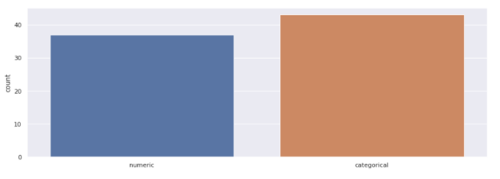
Here as we see that the number of categorical features actually exceeds the number of numeric features which shows how important these features are. Here we have chosen One hot encoding to convert these categorical features into numerical.

data = pd.get_dummies(data)

After this operation, our original 80 features have been expanded to 314 features. Basically, each label of a categorical feature turns into a new feature with binary values(1 for present and 0 for not present). Now we would split our combined data into training and testing data to do some exploratory analysis on our training data.

train = data[:1460].copy()
test = data[1460:].copy()
train['SalePrice'] = y

Exploratory Data Analysis & Outliers Detection

We would first extract the top-features from our training dataset that have the highest correlation with the Sale Price.

top_features = train.corr()[['SalePrice']].sort_values(by=['SalePrice'],ascending=False).head(30)
plt.figure(figsize=(5,10))
sns.heatmap(top_features,cmap='rainbow',annot=True,annot_kws={"size": 16},vmin=-1)

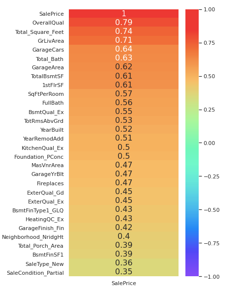
Thus we have extracted the top 30 features having the highest positive correlation with the SalePrice in descending order. Now we would plot some of these features against SalePrice to find outliers in our dataset.

def plot_data(col, discrete=False):
    if discrete:
        fig, ax = plt.subplots(1,2,figsize=(14,6))
        sns.stripplot(x=col, y='SalePrice', data=train, ax=ax[0])
        sns.countplot(train[col], ax=ax[1])
        fig.suptitle(str(col) + ' Analysis')
    else:
        fig, ax = plt.subplots(1,2,figsize=(12,6))
        sns.scatterplot(x=col, y='SalePrice', data=train, ax=ax[0])
        sns.distplot(train[col], kde=False, ax=ax[1])
        fig.suptitle(str(col) + ' Analysis')

This is the plot function that we would use to plot graphs of various features.

OverallQual

plot_data('OverallQual',True)

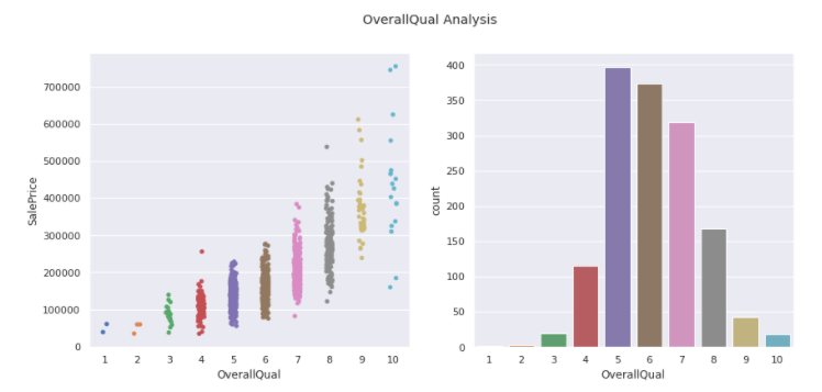
We see there are two outliers with 10 overall quality and sale price less than 200000.

train = train.drop(train[(train['OverallQual'] == 10) & (train['SalePrice'] < 200000)].index)

Thus we dropped these outliers from our dataset. Now we move on to analyze another feature.

Total_Square_Feet

plot_data('Total_Square_Feet')

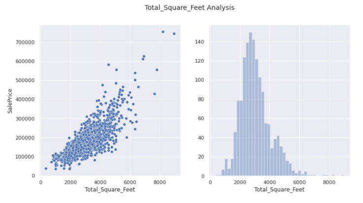
This seems more or less appropriate distribution with no outliers whatsoever.

GrLivArea

plot_data('GrLivArea')

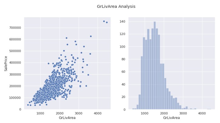
Again no outliers can be eliminated.

Total_Bath

plot_data('Total_Bath')

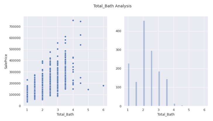
Here we see two outliers that have Total_Bath more than 4 but with sale price less than 200000.

train = train.drop(train[(train['Total_Bath'] > 4) & (train['SalePrice'] < 200000)].index)

Thus we removed these outliers.

TotalBsmtSF

plot_data('TotalBsmtSF')

Here as well we see 1 clear outlier that has TotalBsmtSF more than 3000 but sale price less than 300000.

train = train.drop(train[(train['TotalBsmtSF'] > 3000) & (train['SalePrice'] < 400000)].index)

train.reset_index() # To reset the index

Now that we have taken care of the top features of our dataset we would further remove outliers using the Isolation Forest Algorithm. We use this algorithm since it would be difficult to go through all the features and eliminate the outliers manually but it was important to do it manually for the features that have a high correlation with the SalePrice.

clf = IsolationForest(max_samples = 100, random_state = 42)
clf.fit(train)
y_noano = clf.predict(train)
y_noano = pd.DataFrame(y_noano, columns = ['Top'])
y_noano[y_noano['Top'] == 1].index.values

train = train.iloc[y_noano[y_noano['Top'] == 1].index.values]
train.reset_index(drop = True, inplace = True)
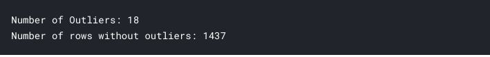
print("Number of Outliers:", y_noano[y_noano['Top'] == -1].shape[0])
print("Number of rows without outliers:", train.shape[0])

We would finally use Standard Scalar from sklearn to scale our data.

X = train.copy()
X.drop(['SalePrice'],axis=1,inplace=True) # Dropped the y feature
y = train['SalePrice'].values

This takes care of our dataset preprocessing and we are finally ready for the next step, which is modeling our data.

MODELLING

We would use Random Search Algorithm from Keras for hyper-parameter tuning of the model.

def build_model(hp):
    model = Sequential()
    for i in range(hp.Int('layers', 2, 10)):
        model.add(Dense(units=hp.Int('units_' + str(i),
                                            min_value=32,
                                            max_value=512,
                                            step=32),
                               activation='relu'))
    model.add(Dense(1))
    model.compile(
        optimizer=Adam(
            hp.Choice('learning_rate', [1e-2, 1e-3, 1e-4])),
        loss='mse',
        metrics=['mse'])
    return model

tuner = RandomSearch(
    build_model,
    objective='val_mse',
    max_trials=10,
    executions_per_trial=3,
    directory='model_dir',
    project_name='House_Price_Prediction')
 
tuner.search(X[1100:],y[1100:],batch_size=128,epochs=200,validation_data=validation_data=(X[:1100],y[:1100]))

model = tuner.get_best_models(1)[0]

The above code is used for tuning the parameters so that we can generate an effective model for our dataset. After running the above code, I got the hyper-parameters that would give me the most effective results for my dataset. I have written a separate function to show this model since running the above code would take a lot of time.

def create_model():
    # create model
    model = Sequential()
    model.add(Dense(320, input_dim=X.shape[1], activation='relu'))
    model.add(Dense(384, activation='relu'))
    model.add(Dense(352, activation='relu'))
    model.add(Dense(448, activation='relu'))
    model.add(Dense(160, activation='relu'))
    model.add(Dense(160, activation='relu'))
    model.add(Dense(32, activation='relu'))
    model.add(Dense(1))
    # Compile model
    model.compile(optimizer=Adam(learning_rate=0.0001), loss = 'mse')
    return model
model = create_model()
model.summary()

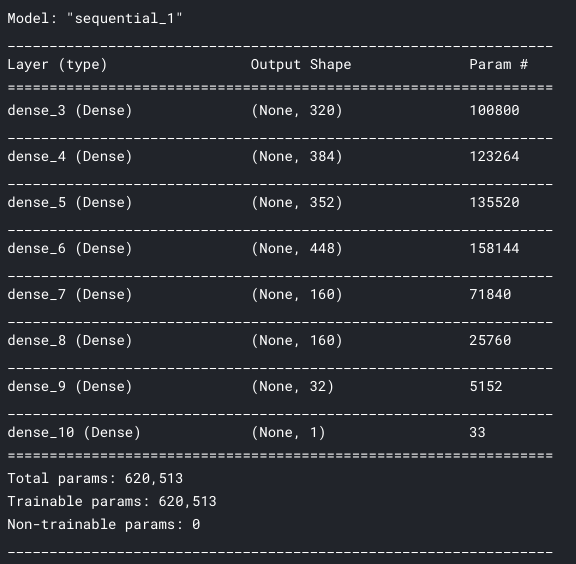
We would be using early stopping callback and would use 1/10th of the training data as validation to estimate the optimum number of epochs that would prevent overfitting

early_stop = EarlyStopping(monitor='val_loss', mode='min', verbose=1, patience=10)
history = model.fit(x=X,y=y,
          validation_split=0.1,
          batch_size=128,epochs=1000, callbacks=[early_stop])
losses = pd.DataFrame(model.history.history)
losses.plot()

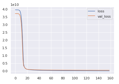
This code shows an early stop at around 160 and since we only used 90% of our training data, therefore we would add 10 to it as a rough estimate and take the number of epochs as 170. Thus we would again reset our model and train our model on the complete training dataset.

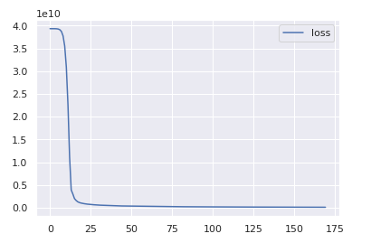
model = create_model() # Resetting the model.
history = model.fit(x=X,y=y,
          batch_size=128,epochs=170)
losses = pd.DataFrame(model.history.history)
losses.plot()

Prediction and Evaluation

We would now run our model against the testing dataset. But before that we need to scale the testing data in the same way as we did for the training data and for that, we would again make use of the StandardScaler function from Sklearn.

X_test = scale.transform(test) # Scaling the testing data.
result = model.predict(X_test) # Prediction using model
result = pd.DataFrame(result,columns=['SalePrice']) # Dataframe
result['Id'] = test['Id'] # Adding ID to our result dataframe.
result = result[['Id','SalePrice']]
result.head()

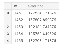
Thus we have got our result which we can submit to kaggle to see how well we have performed.

Note: In the end, I would just like to say that Keras is not the most suitable model for this problem since the dataset given in this is not sufficient.

Thank you for reading. This is my first article on Medium and I would love to hear your feedback on it!!

---

House Price Predictions Using Keras was originally published in Towards AI on Medium, where people are continuing the conversation by highlighting and responding to this story.

Published via Towards AI