Modern NLP: A Detailed Overview. Part 1: Transformers

Author(s): Abhijit Roy

Originally published on Towards AI.

In the recent half-decade, we have seen massive achievements in the Natural Language Processing domain front with the introduction of ideas like BERT and GPT. In this article, we aim to dive into the details of the improvement in a step-by-step manner and see the evolution they have brought along.

Attention is All You Need

In 2017, Ashish Vaswani, from Google Brains, along with colleagues from the University of Toronto, presented an idea for sequence-to-sequence tasks like neural language translation and paraphrasing, different from the existing one-word at a time-step approach followed by LSTMs and RNNs.

The issue with the standing architecture of RNNs as detected were:

1. As we added one word at a time, in the case of long sequences, it was hard to retain information. In encoder-decoder structured models using RNN and LSTM, the hidden vectors were passed from one time-stamp to the other. Then, in the final step, we pass the final context vector to the decoder. The hidden context vector passed to the decoder has a greater influence on the last few words as compared to the first few words of the sequence, as the information is faded over time.
2. To remove the issue mentioned in the first point, an attention mechanism was introduced. This suggested that while decoding, we give separate attention to the words in the input sequence. Every word in the input sequence gets a specific attention weightage vector, which is then multiplied by the word vector to create a weighted sum of vectors. But the issue was, as we did this one step at a time, it took too long for the calculations and also didn’t fully irradicate the information loss.

The Idea

Transformers suggested using a concept called self-attention. The model will take in the entire sentence at a time, and then use self-attention to decide how important are the other words in the sentence in the context of the current word. So, compared to the standing recurrent architecture, it has a few advantages:

1. While detecting the weights, we have all the words already so, there is no possibility of information loss, and also, we get the context from both sides. That is, we get to know both the words, previous to the selected word and words following it, which helps to form a better context, rather than the Recurrent structure (except the case of Bi-LSTM).
2. As we have the availability of the full sentence and also, we need to find the importance of all the other words for each word in the sentence, we can do it parallelly for all the words. This saves a lot of processing time and leads to full utilization of processing power.

Self-Attention: The Building Block

Self-attention mechanism tries to find how much other words are important with respect to a particular word, then create a combined context vector, to represent that word. Basically, it means, if you choose a word in the sentence, how much that is related to the other words in the sentence? As we all know, words define the context of the sentence, and the meaning of a word is dependent on that context more often than not. This is a way to find out the context of the sentence and the related words.

To achieve this, it uses three vectors, namely, Query (Qi), Key(Ki), and Value (Vi), for each input word embedding (xi) in the sentence. The length of the embedding vector x is suggested to be 512, according to the paper. To obtain these vectors first three weight matrices are defined: Wq, Wv, and Wk. We multiply each input word vector Xi with the corresponding weight matrix to get the resulting key, query, and value vectors for the given word.

Qi = Xi * Wq

Vi = Xi * Wv

Ki = Xi * Wk

In order to find out the importance of one word xi in the context of the word xj, we need to find the scalar dot product of the key vector Ki corresponding to the word xi and the query vector Qj for the word xj. The dot product result is then divided by the square root of the dimension of vector Ki, which is 8 as the dimension of k is 64 as given by the paper. As suggested by the paper, if we don’t divide, the dot product value goes too big, which leads to softmax values becoming too steep, and thus producing bad gradients for smooth learning.

Once we find out the importance of all the words for a given word, we use softmax on the results of all the words. The softmax provides the final importance of all the individual words such that they all sum up to 1. Next, comes the value Vi vectors for the words, we multiply the vectors Vi with their corresponding importance. The intuition is the value vectors that create the representation of the words, while the importance factors throw weightage for the context of the subject word. If a word has no relation to the context word, its importance value will be very very low, and thus the final product vector will be very low, and we can disregard its significance for the task. Finally, we take the sum of all these weighted value vectors to create the final context vector for that particular word, which we receive from the attention block.

Multi-Head Attention

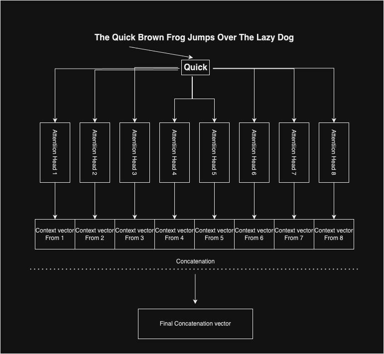
We have seen how attention works and produces context vectors for each word. The authors of the paper used multi-head attention in order to get an unbiased composite context vector. They have used 8 such attention heads, which give 8 different context vectors for a word. The idea is, as each of the internal weight matrices, namely Wq, Wv, and Wk are initialized randomly, the variation of the initialization points in each head may help to capture a range of different features in the context vectors.

Finally, for each word, we have 8 context vectors, which we concatenate together to get the representative context vector for a given word.

The Self-Attention Block: Bringing It All Together

Whatever we have discussed till now is based on one particular word in the sentence, but we do need to think about all the words in the sentence and make the system parallel.

The paper suggests we use embeddings of length 512 to represent each word in the sentence. Now, we already know, for NLP tasks, we usually need to use zero-padding to equalize the sentence length. Next, we stack all the 512-dimensional word vectors on top of each other, and as there is a fixed number of words in a sentence, we get a fixed dimensional 2D vector to represent the entire sentence, which is sent through the entire attention mechanism.

Once we get the combined context vector for all the words, it is multiplied by another weight matrix, which concentrates the learning and reduces the dimension of the vector.

Transformer: The Architecture

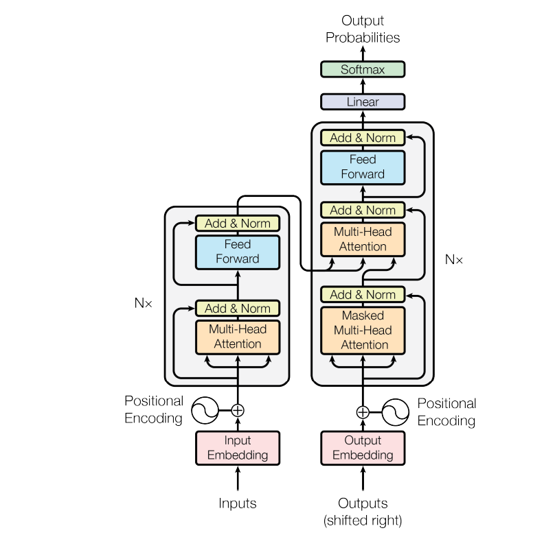
The Transformer also follows a standard Encoder-Decoder architecture. For the sake of easy and better learning, the dimension of the word vectors and outputs of layers are all kept at 512. The learning of the model is done in a auto-regressive manner, i.e., words are produced one by one, and for prediction of the (t+1) th word, we attach the output of the t-th word with the input and feed it to the model.

Encoder: The authors have used modules with 2 sub-layers. The first layer contains Multi-head Attention, which we have discussed above, and the second sub-layer is a fully connected feed-forward layer. The feed-forward layer consists of 2 connected normal neural network layers. The input and output of the feed-forward layers are of dimension 512, but the internal dimensionality is of 2048, i.e, the number of nodes in the internal layer is 2048. The fully connected layer uses ReLU activation. The authors have also used an addition and Normalization layer to smooth the learning and avoid information loss as we have seen in several NLP and computer vision cases.

So, the equation becomes

Output = Norm( x + f(x)), where x is the input and f() is the transformation of the layer, which can either be feed-forward or an attention block.

There are 6 such modules in the encoder block.

Decoder: This is very similar to Encoder Block. This also has 6 modules and a similar architecture. The only difference is, in addition to the 2 sublayers already present, the decoder block introduces a 3rd sublayer, which is also an attention layer, but the inputs are masked so that the model can’t use (t+1)th time stamps word as input while predicting the t-th word. The multi-head attention sublayer, without the mask, takes in the value from the corresponding layer’s encoder. So, the layer takes in input from the previous decoder layer and the corresponding encoder layer.

The Attention layer has been used by the model in 3 different ways, according to authors, while training. As we already know, we input three vectors for all the words, Key, Query, and Value, to the attention blocks, the authors have used this to train the model better.

Option 1: In this case, the queries come from the previous decoder layer, and the memory keys and values come from the output of the encoder. This allows every position in the decoder to attend to all positions in the input sequence.

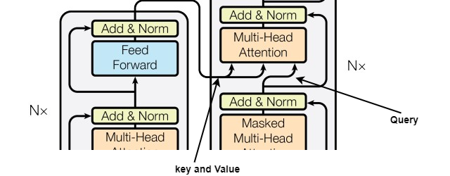
Option 2: In this case, values and queries come from the output of the previous layer in the encoder. Each position in the encoder can attend to all positions in the previous layer of the encoder.

Option 3: In this case, values and queries come from the output of the previous layer in the decoder. Each position in the decoder can attend to all positions in the previous layer of the decoder. Now, this one brings the importance of masked multi-head attention, as the model can’t see words at t+1, the auto-regressive property is preserved.

Finally, the authors have used a linear transformation layer followed by a softmax layer.

Positional Encoding

Apart from the model, this paper also introduced the concept of positional encoding. The issue was, as this paper, does not use recurrent or convolutional networks and is not time step based either, the author felt, there should be something, to signify the positioning of the words, as it plays a major role in expressing the meaning of the sentence.

In order to solve that, the authors brought in two estimations.

where pos is the position of the word, i is the dimension, and dmodel = 512, the input dimension size. The size of the encodings is also kept at dimension 512, so they can be added to the word embeddings easily. The authors have selected these specific functions as, these functions give multiples of the same value after a certain offset, as a result, can be represented as linear functions.

Conclusion

We have learned how transformers works; next, we will learn about other evolutions as well as their implementations as well.

Till then, Happy Reading!!!!

Join thousands of data leaders on the AI newsletter. Join over 80,000 subscribers and keep up to date with the latest developments in AI. From research to projects and ideas. If you are building an AI startup, an AI-related product, or a service, we invite you to consider becoming a sponsor.

Published via Towards AI