


Mastering 10 Regression Algorithms: A Step-by-Step Practical Approach
Last Updated on July 17, 2023 by Editorial Team
Author(s): Fares Sayah
Originally published on Towards AI.
A Hands-On Guide to Understanding and Evaluating Regression Algorithms
Linear Regression is one of the simplest algorithms in machine learning. It can be trained using different techniques. In this article, we will explore the following regression algorithms: Linear Regression, Robust Regression, Ridge Regression, LASSO Regression, Elastic Net, Polynomial Regression, Stochastic Gradient Descent, Artificial Neural Networks (ANNs), Random Forest Regressor, and Support Vector Machines.
We will also examine the most commonly used metrics to evaluate a regression model, including Mean Square Error (MSE), Root Mean Square Error (RMSE), and Mean Absolute Error (MAE).
Import Libraries & Read the Data

Exploratory Data Analysis (EDA)
We will create some simple plots to check out the data. Graphs will help us get acquainted with the data and get intuitions about it, especially outliers which heart Regression models.
<class 'pandas.core.frame.DataFrame'>
RangeIndex: 5000 entries, 0 to 4999
Data columns (total 7 columns):
 # Column Non-Null Count Dtype
--- ------ -------------- -----
 0 Avg. Area Income 5000 non-null float64
 1 Avg. Area House Age 5000 non-null float64
 2 Avg. Area Number of Rooms 5000 non-null float64
 3 Avg. Area Number of Bedrooms 5000 non-null float64
 4 Area Population 5000 non-null float64
 5 Price 5000 non-null float64
 6 Address 5000 non-null object
dtypes: float64(6), object(1)
memory usage: 273.6+ KB

Training a Linear Regression Model
We will begin by training a Linear Regression model but before that, we need to first split up our data into an X array that contains the features to train on, and a y array with the target variable, in this case, the Price column.
After that, we split the data into a training set and a testing set. We will train our model on the training set and then use the test set to evaluate the model.
We created some helper functions to evaluate our Regression models, we explore the theory behind each metric in the next section.
Preparing Data For Linear Regression
Linear regression is been studied at great length, and there is a lot of literature on how your data must be structured to make the best use of the model.
Try different preparations of your data using these heuristics and see what works best for your problem.
- Linear Assumption. Linear regression assumes that the relationship between your input and output is linear. You may need to transform data to make the relationship linear (e.g. log transform for an exponential relationship).
- Remove Noise. Linear regression assumes that your input and output variables are not noisy. This is most important for the output variable and you want to remove outliers in the output variable (y) if possible.
- Remove Collinearity. Linear regression will overfit your data when you have highly correlated input variables. Consider calculating pairwise correlations for your input data and removing the most correlated.
- Gaussian Distributions. Linear regression will make more reliable predictions if your input and output variables have a Gaussian distribution. You may get some benefit from using transforms (e.g. log or BoxCox) on your variables to make their distribution more Gaussian looking.
- Rescale Inputs: Linear regression will often make more reliable predictions if you rescale input variables using standardization or normalization.
1. Linear Regression
Regression Evaluation Metrics
Here are three common evaluation metrics for regression problems:
- Mean Absolute Error (MAE) is the mean of the absolute value of the errors:

- Mean Squared Error (MSE) is the mean of the squared errors:

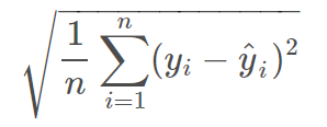
- Root Mean Squared Error (RMSE) is the square root of the mean of the squared errors:
Comparing these metrics:
- MAE is the easiest to understand because it’s the average error.
- MSE is more popular than MAE because MSE “punishes” larger errors, which tends to be useful in the real world.
- RMSE is even more popular than MSE because RMSE is interpretable in the “
y” units.
All of these are loss functions because we want to minimize them.
Test set evaluation:
_____________________________________
MAE: 81135.56609336878
MSE: 10068422551.40088
RMSE: 100341.52954485436
R2 Square 0.9146818498754016
__________________________________
Train set evaluation:
_____________________________________
MAE: 81480.49973174892
MSE: 10287043161.197224
RMSE: 101425.06180031257
R2 Square 0.9192986579075526
__________________________________
2. Robust Regression
Robust regression is a form of regression analysis designed to overcome some limitations of traditional parametric and non-parametric methods. Robust regression methods are designed to be not overly affected by violations of assumptions by the underlying data-generating process.
One instance in which robust estimation should be considered is when there is a strong suspicion of heteroscedasticity.
A common situation in which robust estimation is used occurs when the data contain outliers. In the presence of outliers, least squares estimation is inefficient and can be biased. Because the least squares predictions are dragged towards the outliers, and because the variance of the estimates is artificially inflated, the result is that outliers can be masked.
Random Sample Consensus — RANSAC
Random sample consensus (RANSAC) is an iterative method to estimate the parameters of a mathematical model from a set of observed data that contains outliers when outliers are to be accorded no influence on the values of the estimates. Therefore, it also can be interpreted as an outlier detection method.
A basic assumption is that the data consists of “inliers”, i.e., data whose distribution can be explained by some set of model parameters, though may be subject to noise, and “outliers” which are data that do not fit the model. RANSAC also assumes that, given a (usually small) set of inliers, there exists a procedure that can estimate the parameters of a model that optimally explains or fits this data.
Test set evaluation:
_____________________________________
MAE: 84645.31069259303
MSE: 10996805871.555056
RMSE: 104865.65630155115
R2 Square 0.9068148829222649
__________________________________
====================================
Train set evaluation:
_____________________________________
MAE: 84956.48056962446
MSE: 11363196455.35414
RMSE: 106598.29480509592
R2 Square 0.9108562888249323
__________________________________
3. Ridge Regression
Ridge regression addresses some of the problems of Ordinary Least Squares by imposing a penalty on the size of coefficients. The ridge coefficients minimize a penalized residual sum of squares,

alpha >= 0 is a complexity parameter that controls the amount of shrinkage: the larger the value of alpha, the greater the amount of shrinkage, and thus the coefficients become more robust to collinearity.
Ridge regression is an L2 penalized model. Add the squared sum of the weights to the least-squares cost function.
Test set evaluation:
_____________________________________
MAE: 81428.64835535336
MSE: 10153269900.892609
RMSE: 100763.43533689494
R2 Square 0.9139628674464607
__________________________________
====================================
Train set evaluation:
_____________________________________
MAE: 81972.39058585509
MSE: 10382929615.14346
RMSE: 101896.66145239233
R2 Square 0.9185464334441484
__________________________________
4. LASSO Regression
LASSO Regression is a linear model that estimates sparse coefficients. Mathematically, it consists of a linear model trained with L1 prior as a regularizer. The objective function to minimize is:

Test set evaluation:
_____________________________________
MAE: 81135.6985172622
MSE: 10068453390.364521
RMSE: 100341.68321472648
R2 Square 0.914681588551116
__________________________________
====================================
Train set evaluation:
_____________________________________
MAE: 81480.63002185506
MSE: 10287043196.634295
RMSE: 101425.0619750084
R2 Square 0.9192986576295505
__________________________________
5. Elastic Net
Elastic Net is a linear regression model trained with L1 and L2 prior as regularizers. This combination allows for learning a sparse model where few of the weights are non-zero like Lasso, while still maintaining the regularization properties of Ridge.
Elastic Net is useful when multiple features are correlated with one another. Lasso is likely to pick one of these at random, while Elastic Net is likely to pick both. The objective function to minimize is in this case:

Test set evaluation:
_____________________________________
MAE: 81184.43147330945
MSE: 10078050168.470106
RMSE: 100389.49232100991
R2 Square 0.9146002670381437
__________________________________
====================================
Train set evaluation:
_____________________________________
MAE: 81577.88831531754
MSE: 10299274948.101461
RMSE: 101485.34351373829
R2 Square 0.9192027001474953
__________________________________
6. Polynomial Regression
One common pattern within machine learning is to use linear models trained on nonlinear functions of the data. This approach maintains the generally fast performance of linear methods while allowing them to fit a much wider range of data.
For example, a simple linear regression can be extended by constructing polynomial features from the coefficients. In the standard linear regression case, you might have a model that looks like this for two-dimensional data:

If we want to fit a paraboloid to the data instead of a plane, we can combine the features in second-order polynomials, so that the model looks like this:

The (sometimes surprising) observation is that this is still a linear model: to see this, imagine creating a new variable

With this re-labeling of the data, our problem can be written

We see that the resulting polynomial regression is in the same class of linear models we’d considered above (i.e. the model is linear in w) and can be solved by the same techniques. By considering linear fits within a higher-dimensional space built with these basis functions, the model has the flexibility to fit a much broader range of data.
Test set evaluation:
_____________________________________
MAE: 81174.51844119698
MSE: 10081983997.620703
RMSE: 100409.0832426066
R2 Square 0.9145669324195059
__________________________________
====================================
Train set evaluation:
_____________________________________
MAE: 81363.0618562117
MSE: 10266487151.007816
RMSE: 101323.67517519198
R2 Square 0.9194599187853729
__________________________________
7. Stochastic Gradient Descent
Gradient Descent is a very generic optimization algorithm capable of finding optimal solutions to a wide range of problems. The general idea of Gradient Descent is to tweak parameters iteratively to minimize a cost function. Gradient Descent measures the local gradient of the error function with regards to the parameters vector, and it goes in the direction of descending gradient. Once the gradient is zero, you have reached a minimum.
Test set evaluation:
_____________________________________
MAE: 81135.56682170597
MSE: 10068422777.172981
RMSE: 100341.53066987259
R2 Square 0.914681847962246
__________________________________
====================================
Train set evaluation:
_____________________________________
MAE: 81480.49901528798
MSE: 10287043161.228634
RMSE: 101425.06180046742
R2 Square 0.9192986579073061
__________________________________
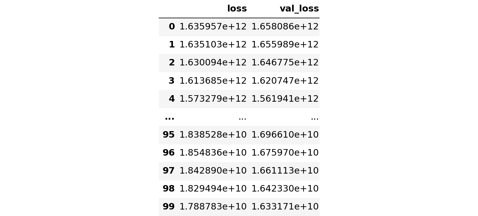
8. Artificial Neural Networks (ANNs)
The benefit of ANNs over simple regression tasks is that the simple linear regression models can only learn the linear relationship between the features and target and therefore cannot learn the complex non-linear relationship. ANNs have the ability to learn the complex relationship between the features and target due to the presence of activation function in each layer.

Test set evaluation:
_____________________________________
MAE: 101035.09313018023
MSE: 16331712517.46175
RMSE: 127795.58880282899
R2 Square 0.8616077649459881
__________________________________
Train set evaluation:
_____________________________________
MAE: 102671.5714851714
MSE: 17107402549.511665
RMSE: 130795.2695991398
R2 Square 0.8657932776379376
__________________________________
9. Random Forest Regressor
Test set evaluation:
_____________________________________
MAE: 94032.15903928125
MSE: 14073007326.955029
RMSE: 118629.70676417871
R2 Square 0.8807476597554337
__________________________________
Train set evaluation:
_____________________________________
MAE: 35289.68268023927
MSE: 1979246136.9966476
RMSE: 44488.71921056671
R2 Square 0.9844729124701823
__________________________________
10. Support Vector Machine
Test set evaluation:
_____________________________________
MAE: 87205.73051021634
MSE: 11720932765.275513
RMSE: 108263.25676458987
R2 Square 0.9006787511983232
__________________________________
Train set evaluation:
_____________________________________
MAE: 73692.5684807321
MSE: 9363827731.411337
RMSE: 96766.87310960986
R2 Square 0.9265412370487783
__________________________________
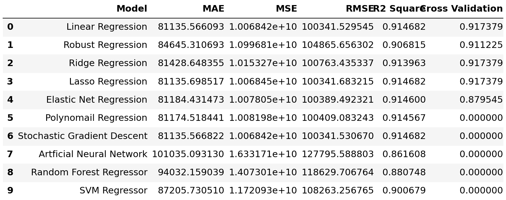
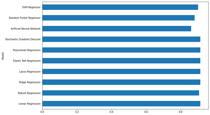
Models Comparison
Summary
In this article, you were introduced to the basics of linear regression algorithms in machine learning. The article covered various aspects of linear regression including:
- Overview of common linear regression models such as Ridge, Lasso, and ElasticNet.
- Understanding the representation used by the linear regression model.
- Explanation of learning algorithms used to estimate the coefficients in the model.
- Key considerations for preparing data for use with linear regression.
- Techniques for evaluating the performance of a linear regression model.
References:
Other Links:
Join thousands of data leaders on the AI newsletter. Join over 80,000 subscribers and keep up to date with the latest developments in AI. From research to projects and ideas. If you are building an AI startup, an AI-related product, or a service, we invite you to consider becoming a sponsor.
Published via Towards AI
Related posts


Popular posts

 for 2021")


Updates

Recent Posts


