N-Dimensional DICOM Volumes With ImageIO

Author(s): Abby Morgan

Originally published on Towards AI.

Visualizing, augmenting, and interacting with high-dimensional DICOM volumes in Python

In this article, we’ll demystify how to access a common format of medical image data, a DICOM file using imageio. We’ll discuss:

• What is a DICOM file?
• Reading a single DICOM file and its metadata
• Reading DICOM volumes
• Visualizing, augmenting, and interacting with DICOM volumes

Let’s dive in!

What is a DICOM file?

DICOM (Digital Imaging and Communications in Medicine) files are the standard format for human medical imaging. DICOM files also contain essential metadata with attributes like patient name, ID, and image pixel data. This format ensures that the medical image data can never be separated from a patient’s metadata by mistake and also that we always have the information we need to properly display the images it contains.

DICOM files with multiple image dataset elements are referred to as “volumes” and are common in a wide range of fields, including radiology, orthopedics, neurology, oncology, veterinary medicine, and more. DICOM files also support various modalities like CT scans, MRIs, and ultrasounds.

Follow along with the full code tutorial in my Google Colab here.

Reading a single DICOM file

Imageio’s imread function takes in a DICOM file and loads it as an image object, which is a type of NumPy array. Once we’ve converted the DICOM file to an imageio image object, we can plot it with matplotlib.pyplot, just as we would any other image array.

# Download data and change working directory
!kaggle datasets download -d salikhussaini49/tcia-chest-ct; unzip tcia-chest-ct.zip; rm tcia-chest-ct.zip
%cd TCIA\ Chest\ CT\ \(Sample\)

import imageio as iio
# Read single DICOM image with imread
im = iio.imread('chest-220.dcm')
# Plot three versions of chest dcm with image transformations
plt.rcParams['figure.figsize'] = (14, 8)
fig, axes = plt.subplots(nrows= 1, ncols= 3)
axes[0].imshow(im, cmap= 'gray')
axes[1].imshow(im, vmin= -200, vmax= 200, cmap= 'gray')
axes[2].imshow(im, vmin= -200, vmax= 200, cmap= 'magma')
axes[0].set_title('Original')
axes[1].set_title('High Contrast')
axes[2].set_title('Colored')
for ax in axes:
 ax.axis('off')
plt.show()

Reading DICOM metadata

One of the most important characteristics of the DICOM file is its structure, which binds the image to its corresponding metadata.

Imageio loads available DICOM metadata into a dictionary that is accessible through the meta attribute. You can also access specific metadata by indexing the meta dictionary with any of the available keys:

# print all metadata keys
print(im.meta.keys())

# print some specific metadata values using their keys
print(im.meta.PatientSex)
print(im.meta.StudyDate

We’ll be taking a look into a few important pieces of metadata in the next section.

Reading a DICOM volume

There are various ways to read a DICOM volume, but in this tutorial, we’ll use ImageIO’s volread() function. This function can load multidimensional datasets directly from a folder of images and aggregate the metadata accordingly.

To plot high-dimensional data, all we have to do is slice it along the desired plane. Plotting slices sequentially can create a “fly-through” effect that helps you visualize the volume as a whole. Below we plot our chest CT scans sequentially:

# plot all five chest DICOM images in one view
fig, axes = plt.subplots(nrows=1, ncols=5)
[axes[x].imshow(vol[x], vmin= -300, vmax = 300) for x in range(5)]
[ax.axis('off') for ax in axes]
plt.show()

Knee CT

We can even make an interactive visualization that steps through the CT scan sequentially using ipywidgets. For this example, we’ll use a volume of knee CT scans that is somewhat larger than the toy dataset we’ve been using so far.

# Download the data from Kaggle
!kaggle datasets download -d abbymorgan/pcir-knee-mri; unzip pcir-knee-mri.zip; rm pcir-knee-mri.zip;

# read in knee volume
knee_vol = iio.volread('PCIR Knee MRI')
# plot interactive knee CT walkthrough
@widgets.interact(knee=(0,26))
def knee_DICOM(knee = 0):
 fig, ax = plt.subplots(1,1, figsize = (8,8))
 ax.imshow(knee_vol[knee,:,:], cmap='bone')
 ax.axis('off')

After using the interactive tool to walk through the full scan, we can isolate a few slices of interest for further evaluation. Let’s say we think we see something interesting around slices 15–20. We can display only those slices with the code below:

# plot slices 15-20
fig, axes = plt.subplots(nrows=1, ncols=5, figsize=(20,15))
for i in list(zip(range(0,5), range(15, 20))):
 [axes[i[0]].imshow(knee_vol[i[1]], cmap= 'bone')]
 [ax.axis('off') for ax in axes]

Slicing different planes

DICOM image data can be 3D or even 4D, but how can we slice the image arrays to view different planes of this information? To answer this question, we’ll first review a few helpful terms.

N-dimensional planes

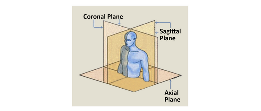
There are many ways to slice a 3D volume into 2D images, but when looking at human anatomy, the three main views are referred to as the axial, coronal, and sagittal planes. However, because most datasets don’t have equal sampling rates across each dimensions, they also often don’t have equal aspect ratios along each dimension. In these cases, we’ll need to stretch the pixels to account for the differences.

But how much should we stretch the pixels and in which directions? In order to calculate this, we’ll have to dive back in to some of our DICOM metadata.

Attribute calculations

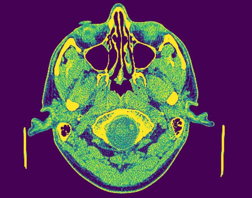
Field of view is the amount of physical space covered by an image. We can calculate the FOV using two other properties, whose values are stored in our DICOM metadata. For this example we’ll use a cranial CT scan. Follow along with the full code here, or download the data here.

1. Array shape: the number of data elements on each axis (metadata key: shape), along each axis.
2. Sampling resolution: the amount of physical space covered by each pixel (metadata key: sampling) along each axis.

# Download data from kaggle
!kaggle datasets download -d abbymorgan/cranial-ct; unzip cranial-ct.zip; rm cranial-ct.zip;

# Read cranial DICOM volume
cranial_vol = iio.volread('Cranial CT')
# Review available metadata
cranial_vol.meta

We can calculate the FOV along each axis by multiplying the shape and sampling attributes for each axis.

Note that the FOV often varies across dimensions (as shown above). This means that the amount of space covered by our image is often not equal across planes, or, in other words, our FOV is often not a perfect cube.

In order to slice different planes of our images, we also need to understand the aspect ratio. The pixel aspect ratio determines how much we need to stretch the pixels in each direction in order to get an appropriately scaled FOV. We can calculate the pixel aspect ratio using the same sampling attribute we used above, which is conveniently stored in the DICOM metadata.

# define sampling resolution along each axis
d0, d1, d2 = cranial_vol.meta.sampling
# define shape along each axis
n0, n1, n2 = cranial_vol.meta.shape

# calculate field of view along each axis
axial_fov = n0 * d0
coronal_fov = n1 * d1
sagittal_fov = n2 * d2
# calculate axial aspect ratio
axial_aspect = d1 / d2
# calculate sagittal aspect ratio
sagittal_aspect = d0 / d1
# calculate coronal aspect ratio
coronal_aspect = d0 / d2
@widgets.interact(brain=(0,225))
def brain_DICOM(brain = 0):
 fig, ax = plt.subplots(1,1, figsize = (8,8))
 ax.imshow(cranial_vol[brain,:,:], vmin= -100, vmax=100)
 ax.axis('off')
# ipywidget wrapper
@widgets.interact(coronal_slice=(0,n1-1),
 sagittal_slice=(0,n2-1))
# walkthrough function
def slicer(coronal_slice=100, sagittal_slice=100):
 fig, ax = plt.subplots(1, 2, figsize=(20, 15))
 # visualize coronal plane
 ax[0].imshow(cranial_vol[:,coronal_slice,:], vmin=-100, vmax=100,aspect= coronal_aspect)
 ax[0].axis('off')
 ax[0].set_title('Coronal')
 ax[0].invert_yaxis()
 # visualize sagital plane
 ax[1].imshow(cranial_vol[:,:,sagittal_slice], vmin=-100, vmax=100,aspect= sagittal_aspect)
 ax[1].axis('off')
 ax[1].set_title('Sagittal')
 ax[1].invert_yaxis()

Notice that the field of view is different in the coronal and sagittal planes than it is in the axial plane, but the scale and proportions of the skull remain consistent. If we hadn’t adjusted the aspect ratio, our coronal and sagittal views would appear stretched. Below we plot a sagittal image with the original unadjusted axial aspect ratio (left), and another image with the corrected sagittal aspect ratio (right).

Wrap up

Thanks for making it all the way to the end of this article, and I hope you found it useful! Feel free to leave me a comment if you have any questions, and stay tuned for more content!

Follow along with the full code tutorial in my Google Colab here.

Feel free to check out some of my other content below!

Join thousands of data leaders on the AI newsletter. Join over 80,000 subscribers and keep up to date with the latest developments in AI. From research to projects and ideas. If you are building an AI startup, an AI-related product, or a service, we invite you to consider becoming a sponsor.

Published via Towards AI