Improving Data Labeling Efficiency with Auto-Labeling, Uncertainty Estimates, and Active Learning

Last Updated on September 13, 2021 by Editorial Team

Author(s): Hyun Kim

In this post, we will be diving into the machine learning theory and techniques that were developed to evaluate our auto-labeling AI at Superb AI. More specifically, how our data platform estimates the uncertainty of auto-labeled annotations and applies it to active learning.

Before jumping right in, it would be useful to have some mental buckets into which the most popular approaches can be categorized. In our experience, most works in deep learning uncertainty estimation fall under two buckets. The first belongs to the category of Monte-Carlo sampling, having multiple model inferences on each raw data and using the discrepancy between those to estimate the uncertainty. The second method models the probability distribution of model outputs by having a neural network learn the parameters of the distribution. The main intention here is to give breadth to the kind of techniques we explored and hope to offer some clarity on how and why we arrived at our unique position on the subject. We also hope to effectively demonstrate the scalability of our particular uncertainty estimation method.

1. A quick review of the efficacy of Auto-labeling

Before we dive into the various approaches to evaluate the performance of auto labeling, there is a note of caution to be exercised. Auto-label AI, although extremely powerful, cannot always be 100% accurate. As such, we need to measure and evaluate how much we can trust the output when utilizing auto labeling. And once we can do it, the most efficient way to use auto-labeling is then to have a human user prioritize which auto-labeled annotation to review and edit based on this measure.

Measuring the “confidence” of model output is one popular method to do this. However, one well-known downside to this method is that confidence levels can be erroneously high even when the prediction turns out to be wrong if the model is overfitted to the given training data. Therefore, confidence levels cannot be used to measure how much we can “trust” auto-labeled annotations.

In contrast, estimating the “uncertainty” of model output is a more grounded approach in the sense that this method statistically measures how much we can trust a model output. Using this, we can obtain an uncertainty measure that is proportional to the probability of model prediction error regardless of model confidence scores and model overfitting. This is why we believe that an effective auto-label technique needs to be coupled with a robust method to estimate prediction uncertainty.

2. Method 1: Monte-Carlo Sampling

One possible approach to uncertainty estimation proposed by the research community is obtaining multiple model outputs for each input data (i.e. images) and calculating the uncertainty using these outputs. This method can be viewed as a Monte-Carlo sampling-based method.

Let’s take a look at an example 3-class classification output below.

y1 = [0.9, 0.1, 0]

y2 = [0.01, 0.99, 0]

y3 = [0, 0, 1]

y4 = [0, 0, 1]

Here, each of the y1 ~ y4 is the model output from four different models on the same input data (i.e. the first model gave the highest probability to class #1, etc.). The most naive approach would be using four different models to obtain these four outputs, but using Bayesian deep learning or dropout layers can give randomness to a single model and allow us to obtain multiple outputs from a single model.

A specific type of a Monte-Carlo based method is called Bayesian Active Learning by Disagreement (BALD) [1, 2]. BALD defines uncertainty as following:

uncertainty(x) = entropy(Avg[y1, … , yn]) – Avg[entropy(y1), … , entropy(yn)]

Like our example output above, BALD assumes we can obtain multiple outputs (y1 ~ yn) for a single input data (x). For example, x can be an image and each y can be a multi-class softmax output vector.

According to the BALD formulation, a model prediction has low uncertainty only when multiple model outputs assign a high probability to the same class. For example, if one model output predicted a “person” class with a high probability and another model output predicted a “car” class with a high probability, then the combined uncertainty would be very high. Similarly, if both models put approximately the same probability to both a “car” class and “person” class, the uncertainty would be high. Seems reasonable.

However, one downside to using a Monte-Carlo sampling approach like BALD for estimating auto-label uncertainty is that one needs to create multiple model outputs for each input data leading to more inference computation and longer inference time.

In the next section, we’ll take a look at an alternative approach that remedies this problem.

3. Method 2: Distribution Modeling

Let’s assume that the model prediction follows a particular probability distribution function (PDF). Instead of having a model optimize over prediction accuracy, we can have the model directly learn the prediction PDF.

If we do so, the neural network output will not be a single prediction on input data but rather the parameters that define or determine the shape of the probability distribution. Once we obtain this distribution, we can then easily obtain the final output y (i.e. the softmax output) by sampling from the probability distribution described by these parameters. Of course, we could Monte-Carlo sample from this distribution and calculate the model uncertainty as we did in the section above but that would beat the purpose of uncertainty distribution modeling.

By using a Distribution Modeling approach, we can directly calculate the output variance using well-known standard formulas for the mean and variance (or other similar randomness measures) of the distribution.

Because we only need one model prediction per data to calculate the auto-label uncertainty, this method is computationally much more efficient than Monte-Carlo during inference time. Distribution modeling, however, has one caveat. When a model directly learns the probability distribution, the class score y is probabilistically defined and thus the model has to optimize over the “expected loss”. Oftentimes this makes an exact computation impossible or the closed-form equation may be extremely complicated, meaning it can be inefficient during training time.

Luckily, this is not an issue in a practical sense because for neural networks the computation time for calculating the loss and its gradient, whether it’s a simple loss or a complex loss formulation, is insignificant compared to the total backward calculation time.

There is an existing work on applying this uncertainty distribution modeling approach to multi-class image classification tasks, called “Evidential Deep Learning” [3]. We’ll take a closer look into this work in the next section.

4. Evidential Deep Learning for Multi-Class Classification

Evidential Deep Learning (EDL) is a type of uncertainty estimation method that uses the uncertainty distribution modeling approach explained above. Specifically, EDL assumes that the model prediction probability distribution follows a Dirichlet distribution.

Dirichlet distribution is a sensible choice for this purpose because of several reasons:

1.) Dirichlet distribution is used to randomly sample a non-negative vector that sums to 1, and is thus suitable for modeling a softmax output.

2.) The formula for calculating the expected loss and its gradient for a Dirichlet distribution is exact and simple.

(For more details on calculating the expected loss of a Dirichlet distribution, take a look at Equations 3, 4 and 5 of the paper [3]. Each equation corresponds to a multinomial distribution, cross-entropy loss and sum-of-squares loss, respectively.)

3.) Most importantly, Dirichlet distribution not only has a formula for calculating the variance measure, but there is also a formula for calculating the theoretical uncertainty measure that falls between 0 and 1.

(This is because we can map the Dempster-Shafer theory of evidence to a Dirichlet distribution. If you are curious, you can read more about this here [4].)

Let’s go one step further into the last point, #3. We can calculate the uncertainty of a Dirichlet distribution with the following formula:

uncertainty(x) = Sum[1] / Sum[1 + z]

where,

• 1 and z are vectors of length N, where N is the number of classes (thus, Sum[1] = N).
• z is the parameter defining the Dirichlet distribution, and is a non-negative vector (it does not have to sum to 1).
• Because Sum[1 + z] ≥ Sum[1] (with the equality being when all elements of z are 0), the uncertainty is always between 0 and 1.

The neural network output z is equal to the Dirichlet distribution parameter, and semantically, the size of each element of the vector z corresponds to the level of certainty for each class.

Let’s visualize the Dirichlet distribution for two cases of z.

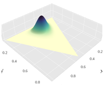
As Sum[z] gets larger, the distribution gets narrower, centered around the mean value.

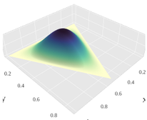
As Sum[z] gets smaller, the distribution gets wider and flattens out, and becomes a uniform distribution when z = 0.

For example, when a given input x is close to the decision boundary (a “hard example”), there is a higher chance that:

1. the model prediction will be incorrect,
2. the model will get a high loss value, and
3. the expected loss increases.

In order to optimize over the expected loss, the model during training learns to reduce the z value so that it can flatten out the prediction probability distribution and reduce the expected loss.

On the flip side, when the input x is far away from the decision boundary (an “easy example”), the model learns to increase z to narrow down the distribution so that it’s close to a one-hot vector pointing to the predicted class.

5. Superb AI’s Uncertainty Estimation

The two types of uncertainty estimation we’ve looked at above, Monte-Carlo methods such as BALD and Uncertainty Distribution Modeling methods such as EDL, are both designed for an image classification problem. And we saw that both methods each have drawbacks: Monte-Carlo method requires multiple outputs from each input and is inefficient during inference time; Uncertainty Distribution Modeling requires that the prediction probability distribution follows a certain known type of distribution.

We have combined these two methods and invented a patented hybrid approach that has been applied to our Auto-label engine. Here are the two best practices for using our Auto-labeling feature and its uncertainty estimation for Active Learning.

Ex. 1) Efficient Data Labeling and QA

One of the most effective ways to use uncertainty estimation is for labeling training data.

A user can first run Superb AI’s Auto-label to obtain automatically labeled annotations as well as the estimated uncertainty. The uncertainty measure is shown in two ways:

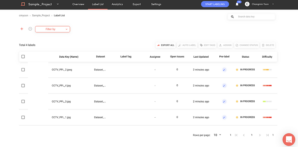
1) Image-level Difficulty — our auto-label engine scores each image as easy, medium or hard. Based on this difficulty measure, a human reviewer can focus on harder images and more effectively sample data for review.

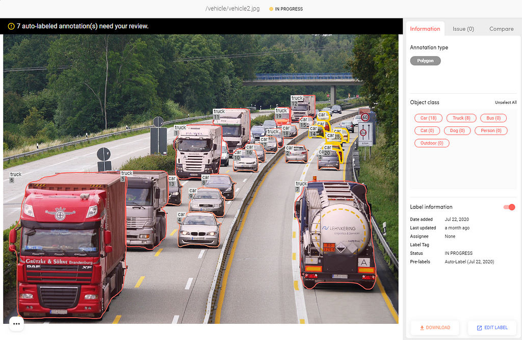
2) Annotation-level Uncertainty — the auto-label engine also scores the uncertainty of each annotation (bounding box, polygon), and requests your review on those that fall below a threshold. In the example below, most of the vehicles were automatically labeled, and you can see that our AI requested user review on the annotations that are smaller or further back in the scene (marked in yellow).

Ex. 2) Efficient Model Training by Mining Hard Examples

Another way to use uncertainty estimation is for efficiently improving production-level model performance.

Most samples in a training dataset, in fact, are “easy examples” and don’t add much to improving the model’s performance. It’s the rare data points that have high uncertainty, or the “hard examples”, that are valuable. Therefore, if one can find “hard examples” from the haystack the model performance can be improved much more quickly.

To illustrate this point, we’ve applied our uncertainty estimation technique on the COCO 2017 Validation Set labels. Here are the results.

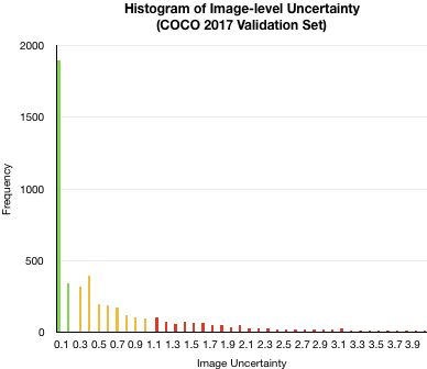
First, we’ve plotted a histogram of image-level uncertainty. As you can see, most of the images have a very low uncertainty below 0.1 and there is a long tail distribution of uncertainty levels up until ~4.0. The green, yellow and red colors indicate how these would appear on our Suite platform as Easy, Medium and Hard.

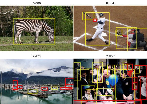
Here’s an illustration of the differences in image-level uncertainty. As the uncertainty measure increases, you can see that the image becomes more complex — more objects, smaller objects and more occlusions between them.

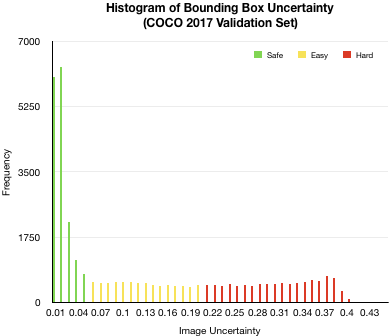
Next, we’ve plotted a histogram of annotation (bounding box) uncertainty. Again, most bounding box annotations have very low uncertainty (below 0.05), and interestingly for this case, the histogram is more or less uniform for uncertainty measures between 0.1 and 0.3.

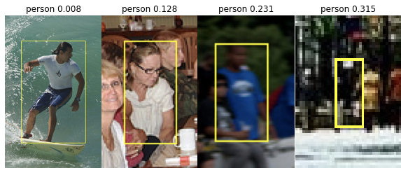
Again, to illustrate the difference in annotation uncertainty, there are four “person class” bounding boxes at varying uncertainty levels above. As the uncertainty increases, you can see that the person is occluded, blurry, and smaller (further back in the scene).

In summary, even one of the most widely used datasets like COCO is heavily centered around easy examples. This will probably be the case for your dataset(s) as well. However, as described in this article, being able to incorporate uncertainty estimation frameworks to quickly identify hard examples near the decision boundary will undoubtedly assist in overall prioritization and active learning.

Coming Soon

In the next part of our Tech Series, we will talk about “Improving Auto-Label Accuracy With Class-Agnostic Refinement” followed by “Adapting Auto-Label AI To New Tasks With Few Data (Remedying The Cold Start Problem)”. To get notified as soon as it is released on Towards AI, please subscribe here.

About Superb AI

Superb AI’s Suite is a powerful training data platform that empowers ML teams to create training data pipelines that are interoperable and scalable. Whether you are building perception systems for autonomous driving, cancer prognostics, or threat detection, Superb AI provides a faster approach to building AI starting with training data management. If you want to try the platform out, sign up for free today!

References

[1] Houlsby, Neil et al. “Bayesian Active Learning for Classification and Preference Learning.” ArXiv abs/1112.5745 (2011).

[2] Gal, Yarin et al. “Deep Bayesian Active Learning with Image Data.” ICML (2017).

[3] Sensoy, Murat et al. “Evidential Deep Learning to Quantify Classification Uncertainty.” NeurIPS (2018).

[4] Jøsang, Audun et al. “Interpreting Belief Functions as Dirichlet Distributions.” Symbolic and Quantitative Approaches to Reasoning with Uncertainty (2007).

---

Improving Data Labeling Efficiency with Auto-Labeling, Uncertainty Estimates, and Active Learning was originally published in Towards AI — Multidisciplinary Science Journal on Medium, where people are continuing the conversation by highlighting and responding to this story.

Published via Towards AI