Harness DINOv2 Embeddings for Accurate Image Classification

Author(s): Lihi Gur Arie, PhD

Originally published on Towards AI.

If you don’t have a paid Medium account, you can read for free here.

Introduction

Training a high-performing image classifier typically requires large amounts of labeled data. But what if you could achieve top-tier results with minimal data and light training?

DINOv2 is a powerful vision foundation model that generates rich image representation vectors, also known as embeddings. Unlike text-based models like CLIP, which focus on semantic alignment, DINOv2 excels at capturing visual structure, texture, and spatial detail — making it ideal for fine-grained image classification tasks in specialized domains such as medical and biological imaging.

In this tutorial, we’ll explore how to use DINOv2 to build a zero-shot classifier using k-Nearest Neighbors (k-NN), and how to significantly boost performance by training a linear layer on top of the extracted features. Thanks to DINOv2’s high-quality embeddings, we can train an accurate classifier using only a small number of labeled images.

The full code is available in the Colab notebook embedded below, ready for you to explore and adapt to your own data.

Background

DINO (short for Distillation with NO labels), developed by Meta, is a method to train vision models in a self-supervised way, without labels. The produced DINO models are powerful vision foundation models capable of extracting rich features from images. By attaching different heads on top of the DINOv2 backbone, the model can be adjusted to different vision tasks, such as image classification, segmentation, depth estimations and more. Although in this tutorial we won’t be training DINO’s backbone, it’s insightful to understand how it was originally trained. If you’re eager to jump into code, you can skip straight to the Code Implementation section.

𝐃𝐈𝐍𝐎𝐯𝟏

The first version of DINO introduced a self-distillation technique where a student network learns to predict the output of a teacher network. Both the teacher and the student share the same architecture: a Vision Transformer backbone (ViT), and a 3-layered MLP (Multi-Layer Perceptron) head. The teacher network was also introduced with centering and sharpening to avoid collapse. During training, the teacher receives large crops (Global Views) of an image, while the student processes both small (Local Views) and large crops of the same image. The crops are processed through the nets, and the student is trying to predict the output of the sharpened (low temperature) teacher. The sharpening is performed by using a low-temperature value in the softmax of the teacher net, to elevate the confidence of the teacher to a dominant dimension, to allow better guidance to the student.

The students’ weights are updated with the cross-entropy cost function, and the teacher’s weights are updated to be the exponential moving average of the student network.

𝐃𝐈𝐍𝐎𝐯𝟐

DINOv2 enhances this original framework by integrating several key improvements. At its core, DINOv2 utilizes dual objectives that work in tandem:

1. Image level objective – Inherited from DINO, this objective encourages the student network to match the teacher’s global image representation. It operates on the class token to capture the holistic view of the image.
2. Patch level objective – Inspired by iBOT, this objective involves masking certain patches in the student input. The student then attempts to predict these masked regions using the surrounding visible patches as context. Cross entropy is calculated between the student and teacher patch features, promoting local feature understanding.

This dual objective approach encourages both a high-level understanding of the image via the image-level objective, and a detailed local perception via the patch-level objective, resulting in richer visual representations.

The final training loss is a weighted sum of the DINO loss and the iBOT loss, effectively balancing global and local learning signals.

In addition, several other optimizations were introduced in DINOv2, including improved normalization and regularization strategies, a multi-resolution training scheme, and training on a high-quality, curated image dataset. You can read more about it (here).

Code Implementation

After exploring the DINO architecture and its backbone training process, in this tutorial we’ll leverage a pre-trained DINOv2 backbone to extract image representation vectors. First, we’ll evaluate its zero-shot performance using a kNN classifier. Then, we’ll improve performance by training a single linear classification layer on top.

Environment Setup

Since we are using Hugging Face to load the pre-trained model, ensure your Hugging Face token is set up in your Google Colab environment.

Next, Install and import the required libraries.

Dataset overview

We’ll use the EMDS-6 microorganisms dataset, which was originally designed for segmentation, and adapt it for classification in this tutorial. The dataset contains 21 microorganism classes that share visually similar features, making it a fine-grained classification task. With only 40 images per class, and just 32 used for training, it also poses a challenging low-data setting.

I’ve pre-split the data into 80% training and 20% validation sets. You can download the prepared version, structured as follows:

EMDS6_Data/
├── train/
│ ├── actinophrys/
│ ├── arcella/
│ └── ...
├── val/
│ ├── actinophrys/
│ ├── arcella/
│ └── ...

Each sub-folder is named after a class and contains PNG images of the respective microorganism. Below is a random sample from the dataset, one image from each of the 21 classes:

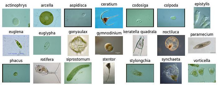
Now that we have downloaded and viewed the dataset, we’ll set up a data pipeline to load and pre-process the images.

Part I – Zero-Shot Classification

In the first part, we’ll examine the zero-shot performance on DINOv2 using a kNN classifier.

Image Data Loading to DINOv2 model

To prepare our data for feature extraction, we use timm’s convenient utilities to define image transforms based on the model’s data configuration. We then create training and validation PyTorch datasets using the ImageDataset class, applying the transforms to each set. Finally, DataLoaders are set up to feed images into the DINOv2 model, ensuring consistent pre-processing and efficient batching of images and labels.

def create_data_loaders(data_dir, batch_size=32, model_name='vit_small_patch14_dinov2', seed=42):
 """
 Create data loaders using timm's transforms and dataset utilities.
 """

 # Set generator with seed for reproducible data loading
 g = torch.Generator()
 g.manual_seed(seed)

 # Create transforms
 data_config = timm.data.resolve_model_data_config(model_name)
 data_config['input_size'] = (3, 518, 518) # DINOv2's native resolution

 train_transform = timm.data.create_transform(**data_config, is_training=True)
 val_transform = timm.data.create_transform(**data_config, is_training=False)

 # Create datasets using timm's Dataset class
 train_dataset = ImageDataset(root=os.path.join(data_dir, 'train'), transform=train_transform)
 val_dataset = ImageDataset(root=os.path.join(data_dir, 'val'), transform=val_transform)

 # Create dataloaders
 train_loader = DataLoader(
 train_dataset,
 batch_size=batch_size,
 shuffle=True,
 num_workers=2,
 pin_memory=True,
 generator=g
 )

 val_loader = DataLoader(
 val_dataset,
 batch_size=batch_size,
 shuffle=False,
 num_workers=2,
 pin_memory=True,
 generator=g
 )

 # Get class mappings
 class_names = train_dataset.reader.class_to_idx
 id2label = {v: k for k, v in class_names.items()}
 label2id = class_names

 print(f"Created data loaders:")
 print(f" Training: {len(train_dataset)} samples, {len(train_loader)} batches")
 print(f" Validation: {len(val_dataset)} samples, {len(val_loader)} batches")
 print(f" Number of classes: {len(class_names)}")

 return train_loader, val_loader, id2label, label2id

# Create data loaders
train_loader, val_loader, id2label, label2id = create_data_loaders(
 data_dir='/content/EMDS6_Data',
 batch_size=32, seed=0
)

Extracting DINOv2 Features

With our DataLoaders ready, the next step is to pass the images through a pre-trained DINOv2 model, to extract rich feature embeddings. By setting num_classes=0, we remove the classification head and obtain raw feature vectors from the backbone.

def extract_features(train_loader, val_loader, model_name='vit_small_patch14_dinov2'):
 """
 Extract features using DINOv2 model from timm.
 """
 device = torch.device("cuda" if torch.cuda.is_available() else "cpu")

 # Create a feature extractor using timm
 model = timm.create_model(
 model_name,
 pretrained=True,
 num_classes=0 
 ).to(device)
 
 model = model.eval()

 # Function to extract features
 def extract_batch_features(loader):
 all_features = []
 all_labels = []

 with torch.no_grad():
 for images, labels in tqdm(loader, desc="Extracting features"):
 images = images.to(device)
 features = model(images)
 all_features.append(features.cpu())
 all_labels.append(labels)

 return torch.cat(all_features, dim=0), torch.cat(all_labels, dim=0)

 # Extract features from train and validation sets
 train_features, train_labels = extract_batch_features(train_loader)
 print(f"Training features shape: {train_features.shape}")

 val_features, val_labels = extract_batch_features(val_loader)
 print(f"Validation features shape: {val_features.shape}")

 return train_features, train_labels, val_features, val_labels

# Extract features
train_features, train_labels, val_features, val_labels = extract_features(
 train_loader, val_loader
)

Zero-Shot Classification with kNN

To assess the quality of the DINOv2 embeddings, we apply a k-Nearest Neighbors (kNN) classifier directly on the extracted features. This simple method doesn’t involve any training — it classifies each validation image based on the closest embeddings from the training set. The result: a kNN accuracy of 83.9% which is quite a decent outcome given the challenge of distinguishing between 21 fine-grained classes. That said, we can push the performance further by training a linear classifier on top.

Part II – Training a Linear Classifier Head

While kNN classifies based on the distance between features, it doesn’t adjust to the specific decision boundaries that separate the classes on our dataset. By training a linear classifier with the embeddings as inputs, we can better shape the feature space to match our dataset and better separate the classes.

Feature DataLoader Setup

To efficiently load the data in batches during training, we create a new set of DataLoaders to handle the previously extracted DINOv2 embeddings.

def create_feature_dataloaders(train_features, train_labels, val_features, val_labels, batch_size=64, seed=42):
 """
 Create data loaders for pre-extracted features.
 """
 # Set generator with seed for reproducible data loading
 g = torch.Generator()
 g.manual_seed(seed)

 # Use timm.data.Dataset for feature datasets
 train_dataset = TensorDataset(train_features, train_labels)
 val_dataset = TensorDataset(val_features, val_labels)

 train_loader = DataLoader(
 train_dataset,
 batch_size=batch_size,
 shuffle=True,
 num_workers=0,
 pin_memory=True,
 generator=g
 )

 val_loader = DataLoader(
 val_dataset,
 batch_size=batch_size,
 shuffle=False,
 num_workers=0,
 pin_memory=True,
 generator=g
 )

 print(f"Created feature dataloaders:")
 print(f" Training: {len(train_dataset)} samples, {len(train_loader)} batches")
 print(f" Validation: {len(val_dataset)} samples, {len(val_loader)} batches")

 return train_loader, val_loader

# Create feature dataloaders
train_feature_loader, val_feature_loader = create_feature_dataloaders(
 train_features, train_labels, val_features, val_labels, seed=0
)

Defining a Linear Classification Head

We define a simple PyTorch model consisting of a dropout layer followed by a fully connected linear layer. The input to the model is a DINOv2 feature vector, and the output is a class score for each microorganism category. This lightweight head is easy to train and sufficient to achieve strong results.

class DINOv2Classifier(nn.Module):
 """Linear classifier for DINOv2 features."""
 def __init__(self, input_dim, num_classes):
 super().__init__()
 self.classifier = nn.Sequential(
 nn.Dropout(0.2),
 nn.Linear(input_dim, num_classes)
 )

 def forward(self, x):
 return self.classifier(x)


# Create classifier model
feature_dim = train_features.shape[1]
num_classes = len(id2label)
classifier = DINOv2Classifier(feature_dim, num_classes).to(device)

Training The Classification Head

In this step, we define the training loop parameters and train the linear classification head. The loop keeps track of the best model weights based on validation accuracy.

def train_model(classifier, train_loader, val_loader, num_epochs, lr):
 """Train the classifier on extracted DINOv2 features."""

 # Setup training
 criterion = nn.CrossEntropyLoss()
 optimizer = torch.optim.Adam(classifier.parameters(), lr=lr, weight_decay=1e-5)
 scheduler = CosineAnnealingLR(optimizer, T_max=num_epochs, eta_min=1e-6)
 history = {'train_loss': [], 'train_acc': [], 'val_loss': [], 'val_acc': [], 'lr': []}
 best_val_acc = 0.0

 for epoch in range(num_epochs):
 # Training phase
 classifier.train()
 train_loss, train_correct = 0.0, 0

 for features, labels in tqdm(train_loader, desc=f"Epoch {epoch+1}/{num_epochs} - Train"):
 features, labels = features.to(device), labels.to(device)

 # Forward & backward pass
 outputs = classifier(features)
 loss = criterion(outputs, labels)
 optimizer.zero_grad()
 loss.backward()
 optimizer.step()

 # Track metrics
 train_loss += loss.item() * features.size(0)
 _, predicted = torch.max(outputs, 1)
 train_correct += (predicted == labels).sum().item()

 # Validation phase
 classifier.eval()
 val_loss, val_correct = 0.0, 0

 with torch.no_grad():
 for features, labels in tqdm(val_loader, desc=f"Epoch {epoch+1}/{num_epochs} - Val"):
 features, labels = features.to(device), labels.to(device)

 outputs = classifier(features)
 loss = criterion(outputs, labels)

 val_loss += loss.item() * features.size(0)
 _, predicted = torch.max(outputs, 1)
 val_correct += (predicted == labels).sum().item()

 # Calculate epoch metrics
 train_size, val_size = len(train_loader.dataset), len(val_loader.dataset)
 train_loss, train_acc = train_loss / train_size, train_correct / train_size
 val_loss, val_acc = val_loss / val_size, val_correct / val_size

 # Update the learning rate
 scheduler.step()
 current_lr = optimizer.param_groups[0]['lr']

 # Store metrics
 for key, value in zip(
 ['train_loss', 'train_acc', 'val_loss', 'val_acc', 'lr'],
 [train_loss, train_acc, val_loss, val_acc, current_lr]):
 history[key].append(value)

 # Print results & save best model
 print(f"\nEpoch {epoch+1}/{num_epochs}: train_acc={train_acc:.4f}, val_acc={val_acc:.4f}, lr={current_lr:.6f}")

 if val_acc > best_val_acc:
 best_val_acc = val_acc
 torch.save(classifier.state_dict(), "/content/best_dinov2_classifier.pth")
 print(f"✓ New best model saved: {val_acc:.4f}")

 return history

# Train the classifier
history = train_model(classifier, train_feature_loader, val_feature_loader, num_epochs=20, lr=0.5)

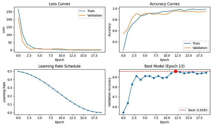
Looking at the training plots below, we observe a clear drop in loss and a strong rise in accuracy during the early epochs, indicating that the model is effectively learning. As training progresses and the learning rate decreases, the model gradually converges and stabilizes. The best-performing model is saved at epoch 13, achieving an impressive validation accuracy of 95.8%, a significant improvement over the zero-shot kNN baseline!

Closing Remarks

In this tutorial, we used DINOv2’s rich embeddings to build an accurate microorganism classifier. Despite the small and challenging dataset, we achieved 83.9% zero-shot accuracy with kNN, and 95.8% by training a simple linear head. DINOv2 is well-suited for scenarios with limited labels and fine-grained visual detail. However, its heavy backbone makes it less suitable for real-time applications or deployment on low-resource edge devices. For tasks that require deeper semantic understanding, Vision-Language Models like CLIP may provide more contextually appropriate embeddings.

Thank you for reading!

Congratulations on making it all the way here! If you enjoyed the tutorial, tap 👍x50 to boost the algorithm’s self-esteem and help more readers find it 🤓

Want to learn more?

• Explore additional articles I’ve written
• Subscribe to get notified when I publish articles
• Follow me on Linkedin

Full Code as Colab notebook:

Join thousands of data leaders on the AI newsletter. Join over 80,000 subscribers and keep up to date with the latest developments in AI. From research to projects and ideas. If you are building an AI startup, an AI-related product, or a service, we invite you to consider becoming a sponsor.

Published via Towards AI