Enhancing Multi-Layer Perceptron Performance: Demystifying Optimizers

Author(s): Anand Raj

Originally published on Towards AI.

Introduction

Optimizers are algorithms or methods used to adjust the attributes of a model, such as its weights and learning rate, in order to minimize the error or loss function during the process of training a machine learning model. The main objective of an optimizer is to find the optimal set of parameters that result in the best performance of the model on the given dataset.

Gradient Descent

Gradient Descent (GD) is a first-order optimization algorithm used to minimize the cost function in machine learning and optimization problems. It iteratively updates the parameters of a model in the direction of the steepest descent of the cost function with respect to those parameters. The algorithm works by calculating the gradient of the cost function at a particular point and then updating the parameters in the opposite direction of the gradient. GD can be computationally expensive, especially for large datasets, as it requires storing and processing the entire dataset in memory for each iteration. Hence, Stochastic Gradient Descent (SGD) was introduced. SGD processes one sample or mini-batch at a time. SGD tends to converge faster and is more computationally efficient, especially for large datasets.

Stochastic Gradient Descent

Stochastic Gradient Descent (SGD) is an optimization algorithm used to minimize a cost function in machine learning. Unlike traditional Gradient Descent (GD), which computes gradients using the entire dataset, SGD updates model parameters using only one training example (or a small subset, called mini-batch) at a time. This makes SGD more computationally efficient and suitable for large datasets.

SGD introduces more noise in parameter updates compared to GD, which can result in more erratic convergence behavior and slower convergence in some cases. Hence, we introduce the concept of momentum.

Code implementation of Optimizers for SGD.

Momentum + SGD

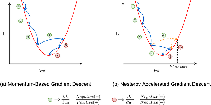
Momentum is an optimization algorithm used to accelerate Gradient Descent (GD) and its variants, such as Stochastic Gradient Descent (SGD), by introducing a momentum term that smooths out the update process and helps overcome local minima. The momentum algorithm maintains a moving average of the gradients and updates the parameters in a direction that aligns with the accumulated gradients.

Momentum is a powerful optimization algorithm that accelerates convergence and helps overcome local minima by introducing momentum into the parameter updates. However, it requires careful tuning of the momentum parameter and may exhibit inertia or increased memory usage in some cases.

Nesterov Accelerated Gradient

Nesterov Accelerated Gradient (NAG) is an optimization algorithm that improves upon the standard Momentum method by taking into account the future gradient. It allows the algorithm to “look ahead” before making a step in the parameter space, resulting in faster convergence and better performance, especially in the presence of noisy gradients.

NAG offers faster convergence, improved accuracy, and less oscillation compared to standard Momentum, but it requires careful tuning of hyperparameters and involves additional computational complexity.

Adagrad

Adagrad, short for Adaptive Gradient Algorithm, is an optimization algorithm designed to adjust the learning rate for each parameter adaptively based on its historical gradients. It is particularly useful in settings where different parameters have vastly different scales or where the gradients of some parameters are sparse.

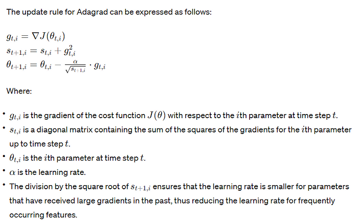
As Adagrad accumulates the squared gradients in the denominator, the learning rates for each parameter decrease monotonically over time. This can lead to excessively small learning rates for parameters associated with frequently occurring features, resulting in slow convergence or premature convergence. It also suffers from inefficiency for non-convex problems, and high memory requirements.

Code implementation of Optimizers for Adagrad.

RMSprop

RMSprop, short for Root Mean Square Propagation, is an optimization algorithm commonly used for training deep neural networks. It addresses some of the limitations of the Adagrad algorithm by adapting the learning rates dynamically based on the magnitude of recent gradients.

It offers advantages such as adaptive learning rates, efficient handling of sparse gradients, and improved convergence speed but may suffer from hyperparameter sensitivity and increased memory requirements.

Code implementation of Optimizers for RMSProp.

Adadelta

Adadelta is an adaptive learning rate optimization algorithm that aims to address some of the limitations of other adaptive algorithms like Adagrad and RMSprop. It dynamically adapts the learning rates based on the magnitude of recent gradients and accumulated gradients over time.

It offers advantages such as no need for a learning rate hyperparameter, memory efficiency, and effective handling of sparse gradients but may be sensitive to initialization parameters and involve computational overhead.

Code implementation of Optimizers for Adadelta.

Adafactor

Adafactor is an adaptive learning rate optimization algorithm that is particularly suitable for training deep learning models with large sparse datasets. It adapts the learning rate based on the statistics of the gradients and the parameter updates.

Its advantages include adaptivity, memory efficiency, and suitability for handling large sparse datasets, but it may require hyperparameter tuning and involve additional computational complexity. While Adafactor shares some similarities with Adagrad in terms of adaptivity and gradient scaling, it introduces several modifications and improvements to enhance its performance, particularly for large-scale optimization problems with sparse datasets.

Code implementation of Optimizers for Adafactor.

Follow-the-Regularized-Leader

FTRL, which stands for Follow-the-Regularized-Leader, is an optimization algorithm commonly used in machine learning for training linear models, particularly in settings where the data is sparse or high-dimensional. FTRL optimizes the regularized loss function by maintaining an adaptive learning rate for each feature.

FTRL (Follow The Regularized Leader) is a powerful online learning algorithm widely used in large-scale machine learning applications, particularly in recommendation systems and online advertising. Its advantages include sparse updates for memory efficiency, built-in L1 and L2 regularization for preventing overfitting, adaptive learning rates based on feature frequency and magnitude, and robustness to noisy and sparse data. However, FTRL comes with certain disadvantages. It involves complex computations compared to simpler algorithms like SGD, requiring careful parameter tuning and potentially leading to higher computational overhead. Understanding and interpreting FTRL can be challenging, making it less intuitive compared to traditional optimization methods. Additionally, FTRL may not be suitable for all optimization problems, particularly those that are non-convex or involve highly non-linear relationships between features and targets.

Code implementation of Optimizers for FTRL.

Adam

The Adam optimizer, short for Adaptive Moment Estimation, is an adaptive learning rate optimization algorithm that computes individual adaptive learning rates for different parameters. It combines the advantages of two other popular optimization algorithms, AdaGrad and RMSProp, by incorporating both first and second moment estimates to adaptively adjust the learning rates.

The Adam optimizer offers several advantages, including adaptive learning rates that adjust for each parameter individually, leading to faster convergence rates and robust performance across various optimization tasks. Its ability to handle noisy or sparse gradients and non-stationary objectives makes it suitable for complex optimization problems. However, these advantages come with some trade-offs. Adam requires additional memory to store separate adaptive learning rates for each parameter, which can be a limitation for memory-constrained environments. Moreover, its performance is sensitive to the choice of hyperparameters, such as learning rate and momentum parameters, and finding the optimal settings may require careful tuning. Additionally, the theoretical properties of Adam are not well understood, particularly in non-convex and non-smooth optimization scenarios, which can make its behavior unpredictable in certain cases.

Code implementation of Optimizers for Adam.

AdamW

AdamW is a variant of the Adam optimizer that incorporates weight decay directly into the update step, addressing the weight decay convergence issue observed in the original Adam optimizer. The mathematical formula for AdamW is similar to Adam, but it adds the weight decay term to the parameter update step, ensuring that the weight decay penalty is applied consistently during optimization. This modification helps stabilize training and prevents the model’s parameters from growing too large during training, improving generalization performance. The advantages of AdamW include faster convergence and better generalization compared to Adam, especially in scenarios with large-scale datasets or complex models. However, like Adam, AdamW requires careful tuning of hyperparameters such as the learning rate and momentum parameters to achieve optimal performance. Additionally, the computational overhead of AdamW may be higher than traditional weight decay methods, as it requires additional calculations during optimization. Despite these considerations, AdamW is widely used in deep learning applications and has demonstrated effectiveness in improving training stability and performance.

Code implementation of Optimizers for AdamW.

Adamax

Adamax is a variant of the Adam optimization algorithm that extends it to be more memory efficient and stable when dealing with large gradients. It is particularly useful in deep learning applications where large datasets and complex models are common.

Its advantages include memory efficiency, stability with large gradients, and adaptive learning rates, but it may require tuning of hyperparameters and involve additional computational complexity.

Code implementation of Optimizers for Adamax.

Nadam

Nadam optimizer is an extension of the Adam optimizer, which combines the ideas of Adam with Nesterov momentum. It stands for “Nesterov-accelerated Adaptive Moment Estimation.” Like Adam, Nadam computes adaptive learning rates for each parameter, but it also incorporates the Nesterov accelerated gradient (NAG) method for faster convergence.

Nadam optimizer combines benefits of Adam and Nesterov momentum, leading to faster convergence and better generalization. Handles non-stationary objectives and sparse gradients well. Automatic adjustment of learning rates for each parameter. Some of the drawbacks include that it requires tuning of hyperparameters such as learning rate, momentum parameters, and epsilon. It might suffer from performance degradation on some tasks compared to simpler optimizers due to increased computational complexity.

Code implementation of Optimizers for Nadam.

Lion

The Lion optimizer is a stochastic-gradient-descent method that uses the sign operator to control the magnitude of the update, unlike other adaptive optimizers such as Adam that rely on second-order moments. This make Lion more memory-efficient as it only keeps track of the momentum.

Code implementation of Optimizers for Lion.

Loss Scale Optimizer

The Loss Scale Optimizer is a technique used in deep learning to mitigate the issue of gradient underflow or overflow, particularly when training with very small or very large gradient values. This approach involves dynamically adjusting the loss scale during training to maintain numerical stability and prevent numerical precision issues, such as vanishing or exploding gradients.

The basic idea behind the Loss Scale Optimizer is to scale the loss function by a certain factor, referred to as the loss scale factor. This factor is typically adjusted dynamically during training based on the magnitude of the gradients encountered. When gradients become too small or too large, the loss scale factor is adjusted accordingly to bring the gradients back within a manageable range.

By using the Loss Scale Optimizer, deep learning models can be trained more effectively and efficiently, as it helps to prevent numerical instability issues that can hinder convergence and degrade performance. However, it’s important to note that implementing the Loss Scale Optimizer requires careful tuning and experimentation to determine the optimal scaling strategy for a given model and dataset.

Overall, the Loss Scale Optimizer is a valuable technique for improving the numerical stability of deep learning training algorithms and enabling the training of more complex and deeper neural networks.

Code implementation of Optimizers for Loss Scale Optimizer.

Learning rate schedules API

Learning rate schedules in machine learning refer to the strategy of adjusting the learning rate during training to optimize the performance of the model. Learning rate schedules can help improve convergence, prevent overfitting, and achieve better generalization. Various learning rate schedules are available in machine learning libraries such as TensorFlow, PyTorch, and Keras, often provided through dedicated APIs.

Here’s an example of how learning rate schedules are typically implemented in TensorFlow and PyTorch:

TensorFlow:

In TensorFlow, learning rate schedules can be implemented using the tf.keras.optimizers.schedules module. You can define a learning rate schedule and pass it to the optimizer during model compilation. Here's an example of using the ExponentialDecay schedule:

import tensorflow as tf

initial_learning_rate = 0.1
lr_schedule = tf.keras.optimizers.schedules.ExponentialDecay(
 initial_learning_rate, decay_steps=10000, decay_rate=0.96, staircase=True
)

optimizer = tf.keras.optimizers.SGD(learning_rate=lr_schedule)

PyTorch:

In PyTorch, learning rate schedules can be implemented using the torch.optim.lr_scheduler module. You can define a scheduler and attach it to the optimizer. Here's an example of using the StepLR scheduler:

import torch
import torch.optim as optim
import torch.optim.lr_scheduler as lr_scheduler

optimizer = optim.SGD(model.parameters(), lr=0.1)
scheduler = lr_scheduler.StepLR(optimizer, step_size=30, gamma=0.1)

In this example, the learning rate will be multiplied by 0.1 every 30 epochs.

These are just a few examples of learning rate schedules available in TensorFlow and PyTorch. Depending on your specific use case, you may choose different schedules such as ReduceLROnPlateau, CosineAnnealingLR, CyclicLR, etc. Each schedule has its own parameters and usage patterns, so it's essential to experiment and choose the one that best suits your needs.

Comparison of All Optimizers — Which one to be chosen when?

Choosing the right optimizer depends on various factors such as the nature of the problem, the architecture of the neural network, the dataset size, and computational resources available. Here’s a brief comparison of popular optimizers and when to choose them:

Stochastic Gradient Descent (SGD):

• Use SGD when you have a large dataset and limited computational resources.
• It’s a good baseline optimizer for simple models and linear regression.

Adam:

• Adam is suitable for most deep learning tasks due to its adaptive learning rate and momentum.
• It works well with large datasets and complex architectures.
• However, it may not converge well with small datasets or on problems with sparse gradients.

AdamW:

• Choose AdamW when training deep neural networks to prevent overfitting.
• It incorporates weight decay directly into the parameter update step, improving generalization performance.

Nadam:

• Nadam combines Nesterov momentum with the adaptive learning rate of Adam.
• It often achieves faster convergence than Adam on deep neural networks.

RMSprop:

• Use RMSprop when dealing with non-stationary objectives or noisy gradients.
• It adapts the learning rate separately for each parameter, making it suitable for online and non-stationary settings.

Adagrad:

• Adagrad is effective for sparse data and convex optimization problems.
• However, it may accumulate the squared gradients over time, leading to a diminishing learning rate.

Adadelta:

• Adadelta is an extension of Adagrad that addresses its diminishing learning rate issue.
• It dynamically adjusts the learning rate based on a moving window of gradient updates, making it suitable for long training sessions.

Adagrad:

• Adagrad is effective for sparse data and convex optimization problems.
• However, it may accumulate the squared gradients over time, leading to a diminishing learning rate.

Adadelta:

• Adadelta is an extension of Adagrad that addresses its diminishing learning rate issue.
• It dynamically adjusts the learning rate based on a moving window of gradient updates, making it suitable for long training sessions.

Adamax:

• Adamax is a variant of Adam that replaces the L2 norm with the infinity norm.
• It is less sensitive to the choice of learning rate hyperparameters.

RMSprop:

• RMSprop is an adaptive learning rate method that divides the learning rate by an exponentially decaying average of past squared gradients.
• It works well for non-stationary objectives and can converge faster than vanilla SGD.

Adafactor:

• Adafactor is an adaptive learning rate method designed specifically for the training of deep neural networks.
• It adapts the learning rate per parameter, using statistics based on the current gradient.

Choosing the right optimizer involves experimentation and tuning hyperparameters based on the specific characteristics of your dataset and model. It’s often recommended to start with Adam or AdamW as they generally perform well across a wide range of tasks and then experiment with other optimizers to see if they offer any improvements for your particular problem.

References

1. Code implementation for all Optimizers: Keras.
2. Lion Optimizer.
3. Optimizers.
4. A Visual Explanation of Gradient Descent Methods.

Hope you liked the article!!!!

You may reach out to me on LinkedIn.

Join thousands of data leaders on the AI newsletter. Join over 80,000 subscribers and keep up to date with the latest developments in AI. From research to projects and ideas. If you are building an AI startup, an AI-related product, or a service, we invite you to consider becoming a sponsor.

Published via Towards AI