Disease Detection with Machine Learning

Last Updated on December 30, 2021 by Editorial Team

Author(s): Daniel Garcia

Introduction

There are many concerns about increasing reliance on technology. Nevertheless, as a society, we continue to push technology to new heights. From how we order food to how we provide healthcare, machine learning, and artificial intelligence continue to help us surpass our wildest dreams. These are some advantages:

1. Improve the diagnosis process

This is very important, especially if early detection and treatment can bring the best results. Using such an algorithm can literally save lives.

Some universities have found through the creation of databases that their artificial intelligence can do as well as doctors in the diagnosis process but also do better in early detection. Artificial Intelligence can also give diagnosis suggestions based on the structured data entered by symptoms, give medication suggestions based on the diagnosis code, and predict adverse drug reactions based on other medications taken.

2. Prevention and rapid treatment of infection

Organizations such as Health Catalyst are using artificial intelligence to reduce hospital-acquired infections (HAI). If we can detect these dangerous infections early, we can reduce the mortality and morbidity associated with them.

3. Crowdsourcing research

With the help of machine learning, the company is working to understand medical issues through crowdsourcing better. Having a larger and more diverse database can help the research be more accurate. In addition, these research methods become more accessible to people from marginalized communities who might otherwise not be able to participate. Finally, participating in research helps patients feel more capable while providing meaningful feedback.

4. Medications

Machine learning has been used to improve medication from anesthesia to breast cancer treatment to daily medication. The famous IBM supercomputer Watson is working with companies such as Pfizer to enhance drug discovery, especially for immune diseases and cancer. Google has been involved for several years and found that machine learning has impressive potential in guiding and improving treatment ideas. Personalized medicine is also the key to treating patients in the future, and machine learning is helping to personalize patients’ feedback on their medications.

Objective

This article aims to contribute to the development of technologies related to Machine Learning applied to medicine by building a project where a neural network model can give a diagnosis from a chest x-ray image of a patient and explain its functioning as simply as possible. So, as we are going to deal mainly with lung-related issues, it’s appropriate to know more about what they really are, in addition to their causes, effects, and history.

Respiratory illnesses are the ones that affect the respiratory system, which is responsible for the production of oxygen to feed the whole body. These illnesses are produced by infections, tobacco, smoke inhalation, and exposure to substances such as redon, asbestos… To this group of illnesses belongs illnesses such as asthma, pneumonia, tuberculosis, and Covid-19.

1. Respiratory illnesses

The first big epidemic belonging to this group of illnesses was the one produced by tuberculosis that affected the lungs. This epidemic was caused by the unacceptable labor conditions of the Industrial Revolution. This health problem was known lots of centuries before but was in that moment when it was first considered a huge health problem that provoked plenty of deaths and remarkable losses. Respiratory illnesses started being treated at the beginning of the XIX century with the invention of the stethoscope by the french doctor René Théophile Hyacinthe. Since that moment, the measures against this kind of illness have been divided into prevention (vaccines) and medical assistance to sick people.

2. Covid-19

Covid-19, which has caused a great impact on our world in the last 2 years, is a branch of the respiratory disease caused by the virus SARS-CoV-2 that affects the respiratory tract. It’s transmitted by the air and the drops emitted when talking, sneezing, or coughing. It appeared for the first time in December 2019 in Wuhan, China, and it rapidly expanded among the whole world until on 11 March of 2020, it was considered a pandemic by the WHO.

Previous attempts

Several decades ago, Artificial Intelligence (AI) became a paradigm that was the basis of a lot of computing projects to be applied to very different fields of our life. One of them was Health, where the AI influence is growing every day. Even more, nowadays nobody knows the limits in this area. Due to the present pandemic worldwide situation, AI has also been applied to Covid-19 disease treatment. In this work, an X-ray thorax image classification system is proposed using Machine Learning. In particular, a Deep Learning prototype was implemented to carry out the corresponding image recognition. More precisely, it is made up of several Convolutional Artificial Neurons layers, as well as a set of dense neuron layers (Multilayer Perceptron).

The classification accuracy obtained was greater than 95% using images never input into our system. In addition, a recent image interpretation belonging to Artificial Vision techniques has been proved, in particular, Grad-CAM, that tries to return the most influential image areas used by a Convolutional Neural Network in a classification problem. As for now, it is not verified if the areas obtained by Grad-CAM are similar to the lung specialist physicians use to consider for the pneumonia diagnosis.

Although several studies have proved that the efficiency of using neural networks is over 95%, some people still think that the human eye is more efficient than AI. Due to the rapid increase of Covid-19 in less than three months, we haven’t got a stock of annotated images. Nevertheless, some researchers have developed a mechanism that can transfer information from generic object recognition to the specific, which is called “DeTraC”. Many researchers consider this method to be easy and quick to apply. The actual efficiency of this method is 95,12% with a sensitivity of 97.91%, a specificity of 91.87%, and a precision of 93.36%.

There are other models like “Alibaba” which works over computed tomography images. This Chinese AI algorithm achieved 96% effectiveness in the detection of Covid-19 pneumonia.

“Covid net”, is a free-access model which lets researchers improve the AI tool that detects SARS-CoV-2. The target of this AI network is to promote the development of highly accurate and practical deep learning solutions to detect COVID-19 cases and accelerate the treatment of those most in need. In conclusion, due to the lack of laboratory analysis kits, in addition to delayed results and limited resources, AI would be a valuable tool for health systems and patients.

How does it work?

To solve the problem of classifying a patient’s chest x-ray image providing an accurate diagnostic, as we discussed earlier, we will use an Artificial Intelligence technique called Convolutional Neural Networks. This kind of network consists of an algorithm that takes an image as input and detects a set of visual features for which it has been trained. The goal here in this particular project is to classify the input image in one of the five possible diagnostics that our model can perform. So the network will use the recognized image characteristics to feed a classical Fully-Connected Neural Network and get a probability prediction for the five different classes to which the image may belong as output. The class with the highest activation (probability) is the one the model selects as the correct diagnostic for the x-ray image.

However, Convolutional Neural Networks can be helpful too in similar computer vision tasks like object and face recognition, image segmentation, self-driving cars, video game automation, weather forecasting, natural language processing (NLP), and even climate change fighting like this initiative that uses machine learning to classify waste using modern Machine Learning algorithms.

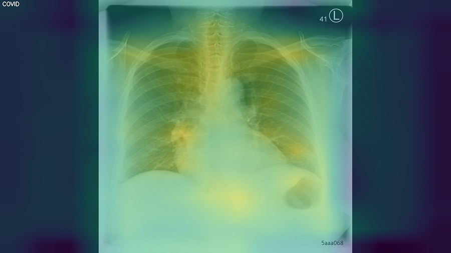
To simplify and visualize in a better manner what the model does, let’s consider this example:

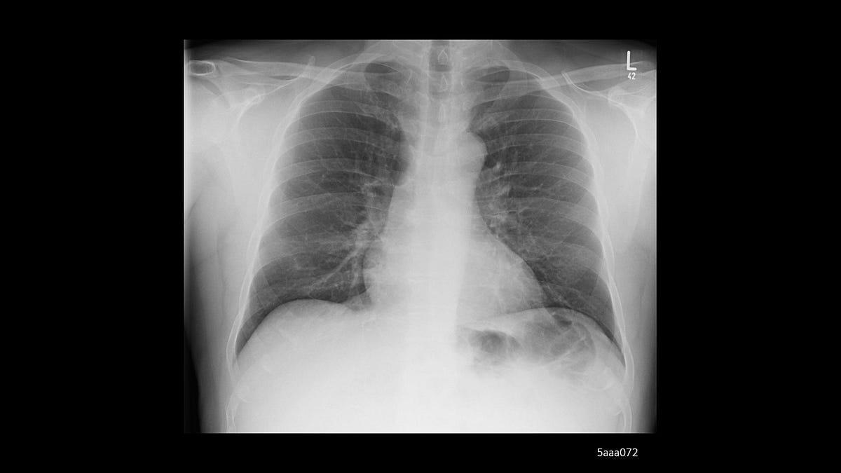
For this image, the model would output the following predictions:

[ 0.001 99.925  0.005  0.067  0.001]
['Bacterial Pneumonia', 'COVID', 'Normal', 'Tuberculosis', 'Viral Pneumonia']

The previous set of values means that the processed image has a 0.001% probability of belonging to the ‘Bacterial Pneumonia’ class, a 99.925% probability of belonging to the ‘Covid’ class, 0.005% probability for ‘Normal’ class, 0.067% probability for ‘Tuberculosis’ class and 0.001% probability for ‘Viral Pneumonia’ class.

As you can see, the class with the highest probability (activation) is the second. Therefore, it indicates that the most correct diagnostic possible is ‘Covid.’ Now, you might be thinking, is the highest value of the predictions set always chosen for the final Classification? Well, it depends on the type of problem you are facing. A threshold number may determine the value from which a class has to be active or not. In this way, dealing with activations is indeed a pretty good approximation of an artificial process for our brain works.

Convolutional networks in deep

First of all, before building our Convolutional Neural Network and the Fully Connected Network of the model that we are going to use to solve the problem, we need to collect a large amount of data in the form of labeled images. With ‘labeled,’ it means that experts in radiology and medicine have already classified the pictures that we get from public datasets.

These are some of the best places to get large amounts of data for artificial intelligence and machine learning projects:

• https://www.kaggle.com/
• https://www.data.gov/
• https://ourworldindata.org/
• https://github.com/awesomedata/awesome-public-datasets
• https://www.google.com/publicdata/directory

In this case, we built a dataset with a total of 23472 image files extracted from the following sites:

– COVID, Pneumonia and Normal

• https://www.kaggle.com/paultimothymooney/chest-xray-pneumonia
• https://www.kaggle.com/tawsifurrahman/covid19-radiography-database

– Tuberculosis

• https://www.kaggle.com/tawsifurrahman/tuberculosis-tb-chest-xray-dataset

Preprocessing data

The part of data preprocessing is crucial on machine learning, where missing, unlabeled, mislabeled, or inconsistent sized data can ruin the training of the model that will learn features from that data. So it’s vital to apply the corresponded technique to ensure the information is ready to be fed into the training process.

The typical way data preprocessing is applied is by using Python libraries, like Keras in this case. For example, if an image file is broken or empty, it should be removed from the dataset to prevent errors. In another case, if a file has a different size than the rest, it should be resized to the correct dimensions. Thereby, there is a data preprocessing technique called’ data augmentation,’ which can sometimes help improve the performance of our model. By rotating, rescaling, moving, and applying a set of transformations to the input images, it can increase the capability of the model to generalize the features it learns.

In the case of diagnosing chest x-ray images, we don’t need to ‘augment’ our dataset due to the small variety of positions that x-ray pictures will have. Nevertheless, we need to need still to preprocess our dataset to make sure the images are ready to be used in the training process.

Here you have an example of how the data is preprocessed in this project:

1. But, first, we import the libraries that we are going to need to develop the project.

import tensorflow as tf
import numpy as np
import matplotlib.pyplot as plt
import itertools
import math
import os

2. The dataset is loaded on ‘GitHub’ so we have to download it by cloning the repository containing it.

!git clone https://github.com/cardstdani/covid-classification-ml.git

3. After cloning the repository, the dataset will be located in the path indicated in the ‘DIR’ variable. The following code splits the primary dataset into a training and a test set with a rate of 90/10, respectively.

This data splitting aims to train the model with the training set and test the accuracy and generalization capability with the test set, so the model will never ‘see’ any data from the test set. Random images are selected from all the dataset classes in the splitting process. Also, the ‘seed’ parameter can change the randomness of the method used to feed the random number generator involved in selecting images that are going to be in each set.

As you can see below, the ‘image_dataset_from_directory’ function from the Keras API has a parameter called ‘image_size,’ which normalizes the size of all images size inside the dataset directory. If some sample has an inconsistent size, it uses the ‘smart_resize’ option to resize it to the ‘image_size’ parameter.

DIR = "/content/covid-classification-ml/Covid19_Dataset"

train_dataset = tf.keras.preprocessing.image_dataset_from_directory(DIR, validation_split=0.1, subset="training", seed=42, batch_size=32, smart_resize=True, image_size=(256, 256))

test_dataset = tf.keras.preprocessing.image_dataset_from_directory(DIR, validation_split=0.1, subset="validation", seed=42, batch_size=32, smart_resize=True, image_size=(256, 256))

4. The number of classes is determined automatically by the number of subfolders inside the main dataset folder, as you can see in this image.

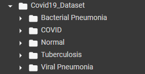
Next, all the dataset’s classes are contained within the ‘class_names’ property of the ‘train_dataset’ object. Finally, the rest of the code improves the performance of the training process. You can find more information about how ‘tf.data.AUTOTUNE’ is optimizing it at the following link.

classes = train_dataset.class_names
numClasses = len(train_dataset.class_names)
print(classes)

AUTOTUNE = tf.data.AUTOTUNE
train_dataset = train_dataset.prefetch(buffer_size=AUTOTUNE)
test_dataset = test_dataset.prefetch(buffer_size=AUTOTUNE)

Artificial Neural Networks (ANN)

As we are working with ‘labeled’ data, it’s essential to know that we face a supervised learning problem. This learning process refers to a set of problems in which the input data is tagged with the result that the algorithm should come up with on its own. That’s the significance of ‘labeled’ data. Usually, these problems are mainly Classification and regression. However, there are other learning methods in Artificial Intelligence, like unsupervised learning. This last procedure consists of a deep learning algorithm that leans patterns on an unlabeled dataset. That means it doesn’t have clear instructions on what it should give as output. Hence, the model automatically finds correlations in the data by extracting useful features and analyzing its structure, all without labeled data. To understand more in-depth about the different learning methods used in machine learning, you can read the following resource:

• https://blogs.nvidia.com/blog/2018/08/02/supervised-unsupervised-learning/

But before explaining its structure and functioning, let’s first know a little more about Artificial Networks (ANN). In general, artificial networks are computational models inspired by a biological brain that constitutes the core of deep learning algorithms. Their main components are neurons, named due to their similarity with the most basic unit that composes a physical neural network. Furthermore, these neurons are disposed of in a series of layers in that each neuron is connected with all the neurons in the next layer. This connection process is sometimes called synapsis. So, with that initial structure, the information can propagate through the input to the network’s output with the aim to make the whole network learn.

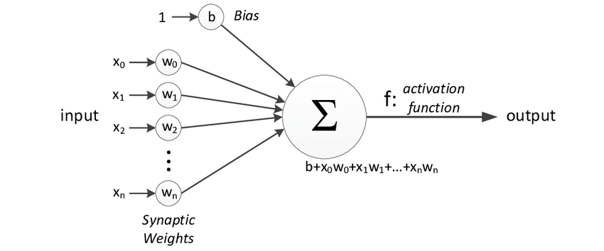
On the above image, you have a representation of a neuron, which is the node that takes n input values x0, x1, x2, xn and multiplies each value with a specific weight number assigned for each input w0, w1, w2, wn. After performing the weighted sum, it adds the results with a bias value and feeds an activation function, whose output will finally be the neuron’s output.

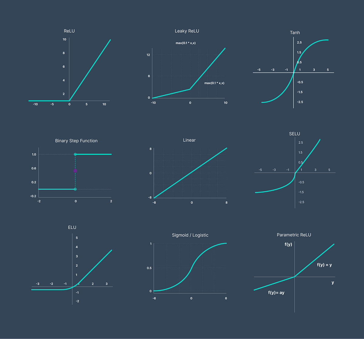
Here you have some of the most used activation functions in Machine Learning. Usually, the two most common are ReLU (Rectified Linear Unit) and Softmax, to calculate probabilities. In general, its primary application is to help the whole network to learn more complex patterns about the data that is input into the network. Although, sometimes, this concept is referred to as nonlinearity. You can learn more about it in the following resource:

• https://medium.com/ml-cheat-sheet/understanding-non-linear-activation-functions-in-neural-networks-152f5e101eeb

To visualize what this process is doing, let’s see one of the most famous cases for an Artificial Neural Network: linear regression.

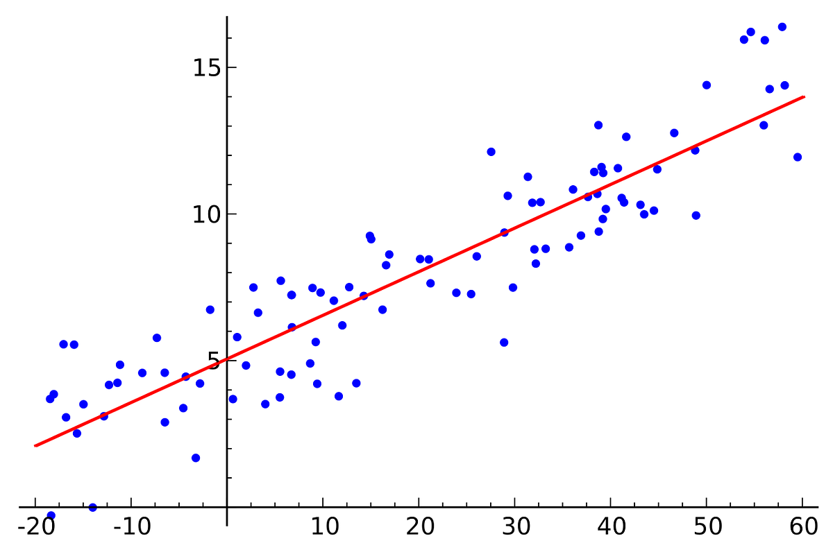
In the above image, you can see a two-dimensional dataset represented as blue points on a chart. Also, you can observe a red line that is the model’s approximation to the data trend. As the formula for a line is y=mx+n, just a neuron with one input value x (his corresponding parameter m) and a bias b (intercept) could be enough to build the model for this particular case due to the linearity of the dataset.

But with a random value selected model, we can’t fit the model’s trend to the dataset’s trend. So we need to train the model to make it learn the pattern that models the data. And the most basic and widely used way to do this is to change the neuron’s parameters until it gives the best result at fitting the data.

The indicator used to evaluate the model’s performance is a loss function that can vary depending on the problem we face. Still, a Mean Squared Error or Mean Absolute Error could help us solve the problem. If you don’t fully understand these terms, ask yourself the following question: How can I calculate how well the model performed in the dataset?

The most intuitive solution would be calculating the average of all the differences between the predictions of the model and the actual values. That’s the Mean Absolute Error. But if you square all the differences while you add the to get the average, you will get the Mean Squared Error. So there are many more ways to calculate the loss that has to be minimized to get an accurate model. If you want to know more, please take a look at this resource:

 

So with a loss function already selected to calculate the model’s performance, we need a method to change the model’s parameters to make it learn while minimizing the loss function. This method is denominated as the optimizer of the model. To intuitively understand how these optimization algorithms work, let’s look at the following animation:

As you can see on the left side, we have our model trying to fit the provided dataset. And on the right, there is a graph with the main parameter of the model on the x-axis, which in this case refers to the slope of the line and the corresponding loss function value for the model’s output on the y-axis. So to optimize (fit) the model parameters and minimize the loss simultaneously, we use an algorithm called Gradient Descent based on an elementary set of steps.

To explain it with an analogy, let’s imagine you are in a pool where the water temperature is different at specific zones. Suppose that your goal is to reach the water’s location with maximum temperature in that pool, but you only have a thermometer. A first approach to reach that point would be an algorithm made with the following steps:

1. First, start at a random point and evaluate in which direction the temperature will be the most.
2. Go forward one step in the direction you found suitable.
3. Repeat this process until you think you have reached your goal.

Similarly, the Gradient Descent algorithm can be defined with the following steps:

1. First, start at a random point and calculate the gradient (derivative) of the function that relates the parameters with the loss of the model at that point.
2. Tweak the parameters in a certain amount (learning rate) to follow the opposite direction of the gradient (slope of derivative). So if the learning rate is too high, it will have difficulties reaching the minimum value. In contrast, it will take a lot of unnecessary time to finish the process if it’s too small.
3. Repeat this process until the process finds the parameters that minimize the loss.

As you can imagine, optimizing a neural network it’s not so simple at all. Furthermore, in more complex models, local minimums might limit the potential of the architecture used to solve the problem. So more advanced techniques and parameters like momentum or Nesterov momentum are added to improve the results of these optimization algorithms. To learn more about optimizers in Machine Learning, visit the following resources:

• https://youtu.be/IHZwWFHWa-w
• https://youtu.be/DDZQYj4AXCA
• https://youtu.be/TudQZtgpoHk

After apprehending the possibilities of an Artificial Neural Network made with one simple neuron, it’s important to visualize how it can be scaled to solve large and complex problems. The below image shows a list of the main network architectures used nowadays in a wide range of real-life applications.

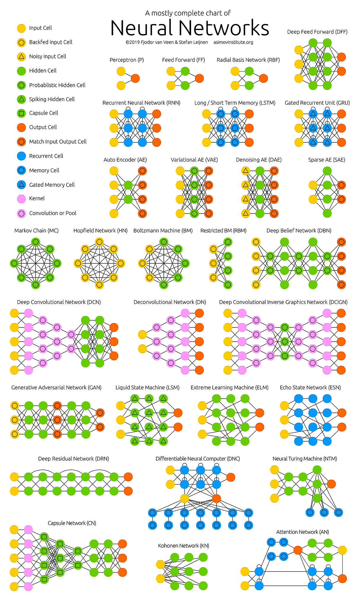
To clarify the concept of Neural Networks without overextending this article, you can learn more about this topic in more detail with the following video series:

Detecting features in images using Convolutions

In this section, we will focus on the problem of making a machine able to ‘see’ things like we humans do in images. First, let’s look at what a feature is and why it’s essential in computer vision with the following example.

With the clearest image, imagine that we want to detect white pixels on a 2×2 grayscale picture like this:

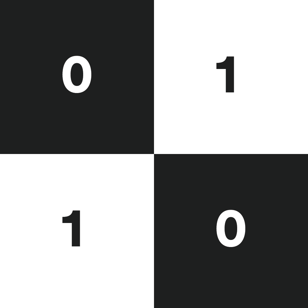
In this case, white pixels 1 are our feature, which we want to detect in the image, and 0 refers to black pixels. So, therefore, a first approach would be comparing all input values with the pixel value of the feature we are searching for and storing the results in a 2×2 matrix full of zeros and ones representing how much our feature is present in each pixel. So when a pixel value of the image is black 0, a zero is stored in the result matrix, also known as a feature map. That approach is called Convolution in computer vision. But to understand it better, let’s learn how it works on a large scale with a bigger image and a more complex feature.

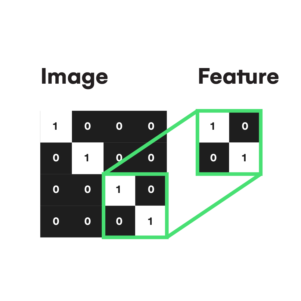
In this case, you can see how the feature we want to detect looks on the right side. So while performing the convolution operation (slicing the filter through all possible positions of the image) in the shown 4×4 image, we will use a filter equal to the feature to know how much a zone of the image is similar to the filter. This process is the key to comprehending how a machine can emulate the human sight sense.

In the first example, we were using a filter of 1×1 size because we wanted to go pixel by pixel detecting a white one, but that isn’t enough when we have pixel dependencies and complex features in images like edges, crosses, shapes, faces, wheels, and any other property that humans can recognize instantly on a picture. So that’s why in the second example, a 2×2 filter is used, and in larger or more complex images, larger filters with more specific number values in them are applied.

To visually understand what’s going on inside a convolution operation, let’s take a look at this GIF:

As you can see, the filter colored in yellow is sliced across all along the image pixels colored in green, starting from the left upper corner and finishing in the right bottom corner of the input image. At the same time, all the coefficients inside it are multiplied by the values of the pixels that it covers. The multiplication operation here results in the best way to compute the ‘presence’ of the feature defined by the filter in the set of image pixels it compares to each step. Once these calculations are done, the resulting numbers are added and divided by the number of pixels the filter has, as if it were an average. Finally, the resulting value is stored in the corresponding position in the feature map, colored in light red.

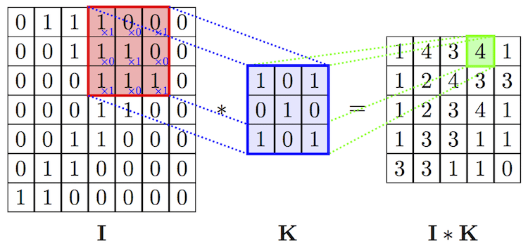
Here you have a more complex example where the filter, also called ‘kernel’ and colored in blue, is used to apply a convolution transformation to the input image represented as the matrix ‘I.’

When processing an image in RGB color mode, which is usual, three filters are applied in the convolution process, one for each color channel representing the picture. Strictly speaking, it’s not three separated filters. There is only one filter, but it has a depth dimension of value three which can reach every color channel in the convolution operation.

At this stage, you may notice that the size of the feature map provided by the Convolution as output is smaller than the original image size. This phenomenon is due to the nature of this algorithm, specifically to the stride property of the kernel, which determines how many pixels it must translate horizontally or vertically in each step. For example, in the following animation, you have a convolution with stride value 2. Notice that the kernel moves 2 pixels each step, causing the feature map to be much smaller than before.

The solution to the ‘problem’ of the output size relapses on adding ‘padding’ to the input image. The padding adds one or several outer frames, usually of zero values, to the matrix representing the picture. So the kernel will have more space to cover the entire image and produce a feature map with the exact dimensions as the provided input.

To summarize, Convolution is an operation that we can apply to images to detect specific patterns and features inside them. The most significant advantage of using Convolutions in this kind of task is that it can recognize an object even when its appearance varies in some way, making it invariant to translations, rotations, changes in light, and size. As you can see below, we have a set of kernels that can detect a different feature which would be helpful when building a convolutional neural network that detects human faces.

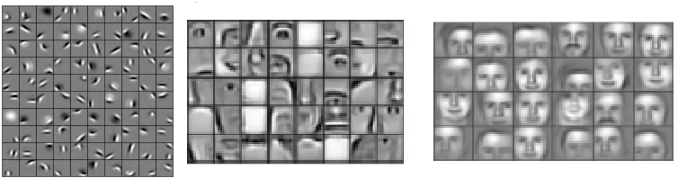
In the left set, we can see that the filters seem too simple to detect faces. Indeed they can only detect straight lines, edges, and maybe basic shapes. But, conversely, in the second and third sets of filters, we can observe a significant increase in their complexity, which now can detect eyes, noses, mouths, ears, hair, whole faces, and so on. That’s because they might be a combination of the initial set. So with a mixture of kernels that detect basic shapes, we can achieve better results at detecting more elaborated image characteristics.

After exposing the functioning of the convolution process, now you may better understand how a machine can extract patterns and features from images to solve a classification or detection problem. If you want to know more about the previously mentioned proceeding, you can use the following resource to answer all the possible doubts about it:

• https://youtu.be/8rrHTtUzyZA

Convolutional Neural Networks Architecture (CNN)

Now, let’s discover and implement a Convolutional Neural Network that will solve our original problem of classifying chest x-ray images in Python using Tensorflow and Keras libraries.

• https://www.tensorflow.org/
• https://keras.io/

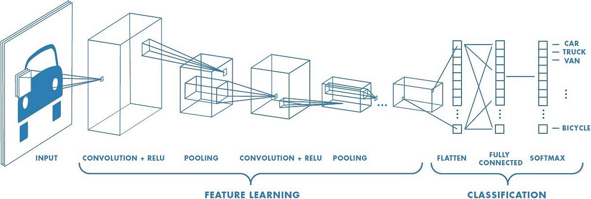
As you can see in the above illustration of the Convolutional Network architecture, it splits into Feature Learning for pattern extraction and Classification for translating the activations of the patterns to the activations of the result classes. That’s so because the main objective is to reduce the images into a shape that is easier to process, maintaining all the necessary information about its pixel dependencies. But sometimes, when you try to build a vast network with a very complex feature learning part, it takes too much time to train and a lot of computer resources that might not be available. So additionally, we will be using a technique called Transfer Learning, in which we replace the convolutional part of our model with an already trained feature extraction model.

Feature Learning

When performing the feature learning section of the network, we are converting our original problem of classifying images to a more straightforward problem of classifying a set of activations where each of them refers to a detected feature in the input image. Furthermore, to adequately reduce the dimensionality of the inputs, we will stack a set of Convolutional layers that apply the Convolution operation over the input image using multiple filters and run an activation function (usually ReLU) at the output feature map to introduce nonlinearity. After each convolution layer is added to the network, a Pooling layer must be stacked on top of it. The Pooling layers are the key to downsampling the output of the Convolutional layers as much as possible without losing essential information about the detected patterns. Its fundamental operating is the same as Convolution, except that Pooling doesn’t perform a weighted sum of the elements covered by the kernel in each step. In contrast, it directly selects the maximum, the minimum, or the average of these elements. These variations of the Pooling operation are called Max, Min, and Average Pooling, respectively, but in Convolutional Neural Networks, Max Pooling is the most used due to its performance.

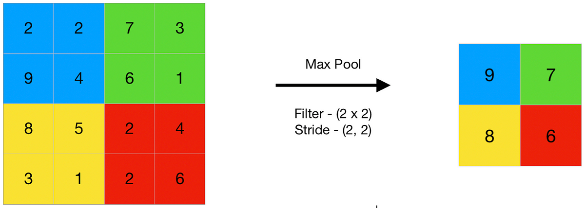
In the above image, you have a representation of a max-pooling operation performed on a 4×4 matrix with a 2×2 kernel using a horizontal and vertical stride of 2. As you can observe, the function is downsampling the original image without breaking its pixel/feature dependency. In this case, you can see it as the input and output colors.

Classification

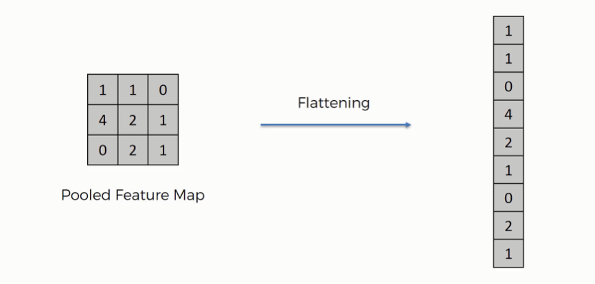
Once the input image features have been detected, the network must transform the shape of the feature maps of the Convolution part and feed a Fully-Connected Network to perform Classification from feature activations. To do that, the most common way to proceed is using a Flatten layer, which takes all the feature maps and returns a one-dimensional list with all their elements stacked, as you can see in the below image.

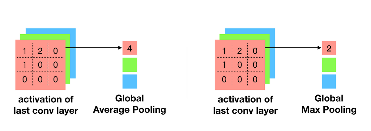
Although this is not the unique way to chain the Convolution and Classification part of the network, it can sometimes cause overfitting problems or simply not the appropriate way to proceed. Such methods like GlobalAveragePooling or GlobalMaxPooling usually solve the overfitting problems caused by the Flatten layer. Its working is very similar to the Pooling that we saw earlier. It performs a Pooling operation over all the feature maps, but this time using a kernel with the exact dimensions as the feature map.

After reshaping the feature maps, a classification network made of stacked Dense layers in which all the nodes are connected with the nodes of the next layer receives the reshaped feature maps and, using a Softmax activation function, returns the set of activations for each class that we are expecting.

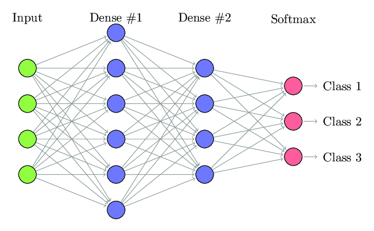
On the above image, you have a representation of the classification part of the network, but if you want to know more in-depth how this entire process works, you can take a look at the following lectures:

Implementation Details

The first thing that we have to do to build the model is to load the pre-trained Convolution part from the Keras API as the base model, without its last layers, from which we will stack the rest of our layers. There are different pre-trained models that we can choose for this kind of feature extraction task, but the one that gives the best performance and takes the least space to work is MobileNetV3Small. You can see a list of available models at the following link. These are trained with imagenet, one of the world’s largest datasets composed of millions of images, and focused on improving the performance of Convolutional Networks.

baseModel = tf.keras.applications.MobileNetV3Large(input_shape=(256, 256,3), weights='imagenet', include_top=False, classes=numClasses)

After having a base convolutional model, we have to set up the Classification part, which is crucial to take advantage of the power of the base model architecture. In this case, we are using a GlobalMaxPooling2D layer to reduce the feature maps dimensionality and fed it into the Dense network, made by a hidden layer of 256 neurons using the ReLU activation function, and an output layer with the same number of neurons as classes in our problem (5). This part of the network also has a Batch Normalization layer that increases the result accuracy of the model and several techniques to reduce overfitting like Dropout and L2 regularizers.

last_output = baseModel.layers[-1].output
x = tf.keras.layers.Dropout(0.5) (last_output)
x = tf.keras.layers.GlobalMaxPooling2D() (last_output)
x = tf.keras.layers.Dense(256, activation = 'relu', kernel_regularizer=tf.keras.regularizers.l2(0.02), activity_regularizer=tf.keras.regularizers.l2(0.02),  kernel_initializer='he_normal')(x)
x = tf.keras.layers.BatchNormalization() (x)
x = tf.keras.layers.Dropout(0.45) (x)
x = tf.keras.layers.Dense(numClasses, activation='softmax')(x)

model = tf.keras.Model(inputs=baseModel.input, outputs=x)

Once the model architecture is built, it needs to be trained and tested to fit the input dataset. So now, we will define the loss function used to evaluate the performance during training and the optimizer algorithm that will tune the model parameters to minimize the loss function. In this case, we use the Stochastic Gradient Descent with an initial learning rate of 0.1 as optimizer and Sparse Categorical Crossentropy, one of the most usual losses in multiclass classification tasks like this. In addition to the loss, we also add the ‘accuracy’ metric, which, as its name indicates, shows the model’s performance in the form of a percentage. However, we can use the loss function as the metric itself, but the main reason for not doing that is the use in which each one is used. For example, the main goal of the loss function is to be minimized during training to optimize the model. At the same time, the metric is an indicator of how well the model is performing, not only in training but in testing and inference too.

model.compile(optimizer=tf.keras.optimizers.SGD(learning_rate=0.1), loss=tf.keras.losses.SparseCategoricalCrossentropy(), metrics=['accuracy'])

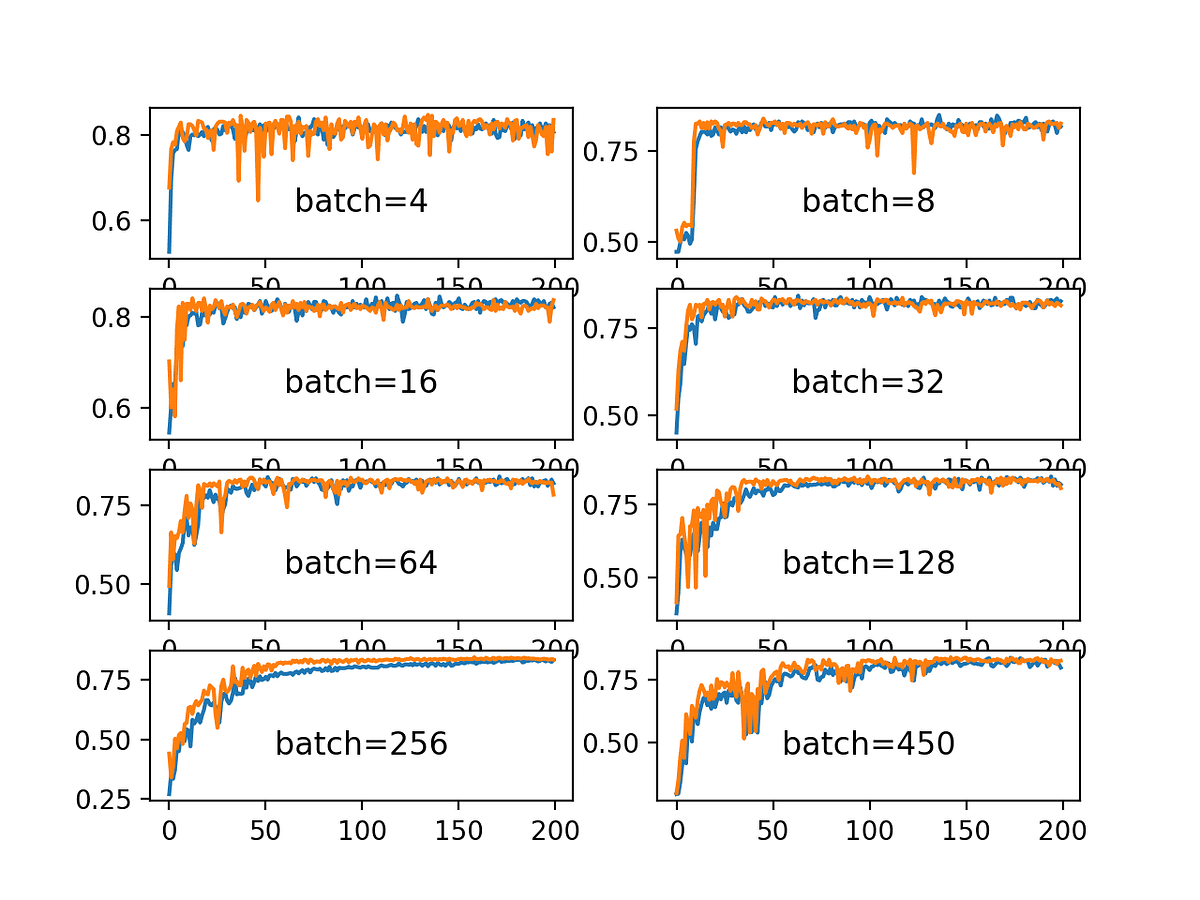
Finally, we define the number of epochs that the model will be training. So in each epoch, the training set is divided into a series of batches with as many images as the batch size (usually 32) and fed into the network to fit its parameters. Thus, the model will train during a single epoch in as many steps as batches the training set can be divided. The objective of that data splitting is to control how stable the learning algorithm trains the network, as you can see in the following image:

And last but not least, we define a callback of the type ‘LearningRateScheduler’ to decrease the learning rate stepwise during training so that it will be divided by ten every six epochs.

epochs = 40
stepDecay = tf.keras.callbacks.LearningRateScheduler(lambda epoch: 0.1 * 0.1**math.floor(epoch / 6))

history = model.fit(train_dataset, validation_data=test_dataset, epochs=epochs, callbacks=[stepDecay])

Now we have a ‘history’ variable created with the fit() function of the model, which contains all the information generated during training, such as loss and accuracy over time, steps per epoch, etc. That data is beneficial when visualizing how the model evolved from a random initialization to a state where it minimizes the loss function and gives a decent accuracy for the task to solve.

Results

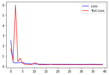
On the above image, you have a graph that shows the loss value of both training and test datasets on the y axis and the current epoch on x. In the beginning, as the model parameters are randomly assigned, the overall loss takes a high value and quickly decreases during the 2–3 subsequent epochs. Then, after it keeps dropping and stabilizing, it finally ends with a fixed value of 0.15 approximately. However, it’s a good signal that both training and test losses end up stabilizing with very similar values. For example, if the training loss had been smaller than the test loss at the end of the training, the model would have overfitted the training data. Thus its generalization capability and performance on unseen data would have been inferior. To understand more in-depth how to interpret this kind of graphs:

After completing the training process, the model ends with an overall accuracy of 95.3%, which is a good value for a classification neural network. Still, it’s not enough to be fully implemented on the sanitary system as one more tool because approximately 5 out of 100 persons would be misdiagnosed. So, to visualize what accuracy means, let’s build a Confusion Matrix and test the final model by making some predictions:

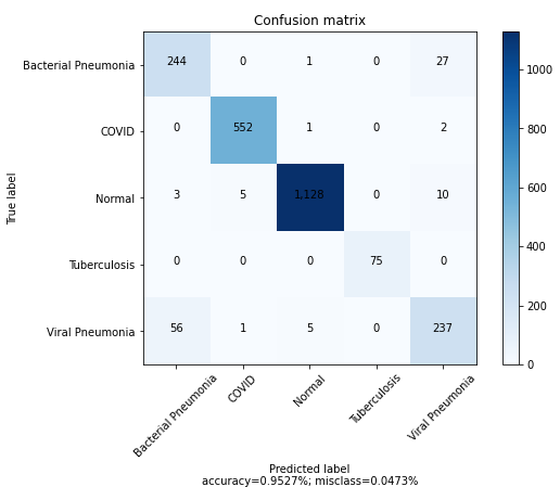
In this confusion matrix, the objective is to visualize the relation between the true labels and the predicted labels of the tested data via plotting it in a matrix graph. So in the y axis, we represent the true labels as rows, and in the x-axis, we place the same labels as before, but this time the columns represent the predicted labels that the model gave as output. The resulting graph for a model that perfectly fits the data should look like an identity matrix, where all the predicted labels of the x-axis match the corresponding actual labels of the y axis. In this case, we can observe a strong tendency to fit the identity matrix of a perfect model. Although, we can see some mispredicted values, especially on the two types of pneumonia, as the accuracy doesn’t reach 100%. That confusion is causing the most issues when fitting the data by reducing the overall accuracy.

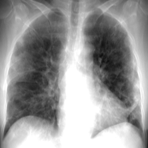
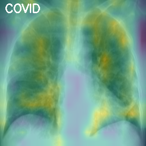
In addition to classifying an image into a class, we can also visualize the activation map that the input image generates on the network neurons. This map represents a significant activation over the features that the network learned to extract with a more yellow color. In contrast, the dark blue color indicates a deficient or null activation. In simple terms, the activation map contains the zones of the image where the model thinks the features will be located.

Conclusion

Once having reached a 95% accuracy, we can conclude that the model does a high number of correct guesses, but there is also much work to be done in order to improve the results of this kind of Machine Learning algorithm on such complex tasks. However, articles like this, which try to explain the power of modern technology applied to the resolution of large-scale problems that couldn’t have been solved before, are useful to provide a better general comprehension of artificial intelligence. Also, knowing more about how the technology we use works improves our ability to use it correctly and contributes to critical and creative thinking development.

Resources

Link to the Colab Notebook with the full implementation: https://github.com/cardstdani/covid-classification-ml/blob/main/ModelNotebook.ipynb

With the collaboration of: Alejandro Pascual, Javier Nieto, Quetzal Gómez, Alberto Ruiz.