
 Logo:
Logo:  Areas Served:
 Classifying NBA Positions by Physical Traits — Part I
Last Updated on June 11, 2024 by Editorial Team
Author(s): Vishnu Regimon Nair
Originally published on Towards AI.
In 2019, NBA teams spent over 3 billion dollars on guaranteed salaries to players in the first three days of free agency. These expensive contracts often lock a player into the team over multiple years. While the athlete receives significant monetary gain, the team attempts to collect the pieces necessary to contend for an NBA championship. These expensive salaries come with substantial risks to the organization. To mitigate the associated dangers of paying an individual so much money, gaining deeper insights into basketball positions and players and how specific statistics and physical attributes contribute to these factors is essential. Who are the best players in the league? Is there a lot of overlap with positions to the point that NBA positions are interchangeable? These are some of the questions that motivated this project. This deeper context and understanding can illuminate how coaches and organizations can fill the positions and roles their roster is currently lacking.
This is the first part of a series called Moneyball for NBA. In the first installment of this series, we explore the potential of physical characteristics, such as height and weight, in classifying NBA player positions using machine learning models.
Table of Contents
· Introduction
· Methodology
· Data Source
· Datasets
· Metadata
· Data cleaning and wrangling steps:
· Exploratory Analysis
· Question 1
∘ Logistic Regression
∘ Polynomial Regression
∘ Support Vector Classifier
∘ Decision Trees
∘ Random Forests
∘ KNN classification
Introduction
This paper utilizes National Basketball Association (NBA) players' statistics based on physical and statistical characteristics to answer three guiding questions:
- Using classification models (Logistic Regression, Classification Trees, Random Forest, Gradient Boosted Trees), can we apply NBA player's weights and heights to classify players based on positions?
- Can we use classification models (Logistic Regression, Classification Trees, Random Forest, Gradient Boosted Trees) to apply NBA players' in-game statistics to classify players based on positions?
- Using PCA and K Means clustering, can we find similar groups of players for each position and discover the most productive players and seasons by position?
The five positions in the NBA are Point Guard (PG), Shooting Guard (SG), Small Forward (SG), Power Forward (PF), and Center. We will classify these players by position using their statistical outputs and physical characteristics. Furthermore, we will implement dimensionality reduction and k-means clustering for each position. This will help us find players with similar play styles within the positions and outstanding players who are the best or most productive in those positions.
Methodology
This section will give a brief overview of the steps to achieve the goal of this paper. First and foremost, the dataset and its source will be acknowledged. Then, the various wrangling and cleaning procedures that occurred will be detailed. This includes downloading, merging, and altering the datasets. Once the data has been treated and organized, we review and discuss exploratory analysis to increase our knowledge and illustrate the significant details of the five positions in the NBA. Some other minor data cleaning may occur where needed.
After familiarising ourselves with the dataset, we will apply a correlation matrix to the data frame’s columns and remove values that exhibit multicollinearity. This will eliminate some extraneous categories from our relatively large number of features.
Following these essential introductory tasks, six classification models will be tested to classify player positions based on height and weight:
- Logistic Regression Analysis
- Polynomial Regression Analysis
- Support Vector Classification
- Decision Tree
- Random Forest Classification
- K Nearest Neighbour Classification
So many different classification methods are being used because we are still determining which method will be the most appropriate for our data. Consequently, we will compare and contrast the best strategies and results.
Once this process is complete, we will complete a similar process to classify players' positions based on in-game statistical categories:
- Logistic Regression Analysis
- Polynomial Regression Analysis
- Support Vector Classification
- Decision Tree
- Random Forest Classification
- K Nearest Neighbour Classification
We completed separate classification techniques for the in-game statistics because we view whether or not physical attributes accurately classify players by position as a separate analysis. Doing these processes separately will substantially increase our understanding of the impacts of physical characteristics and individual skills on deciding positions in the NBA.
Once our classification analysis is complete, we will attempt to answer the last question of our project, which is to find groups of similar players and the best individual season within each position. After separating our data into five separate data frames (one for each position), the final two data science techniques we will employ in our paper to reach this goal are:
- Principal Component Dimensionality Reduction
- K-Means Clustering
Data Source
We found the data for our project at Data World, which records the in-game performance and statistics of NBA basketball players during games. This is licensed under the public domain license. Obtaining a dataset licensed in the public domain proved difficult for this task as most NBA data is at a few centralized locations. Luckily, Data World has a dataset under the public domain license, which means you can use it with no restrictions. Finding a suitable license for the type of data you want to analyze is essential so there aren’t any data licensing issues later on.
Public Domain materials are works that are free from intellectual property laws. There are no restrictions for individuals to use these works, nor are permissions necessary. Works within the Public Domain can never be owned by any individuals. — Source
Metadata
This section will highlight the variables essential to our research and whether they are continuous or discrete. Due to the large number of independent variables (20), we are breaking them into subsections.
Dependent Variable:
NBA Positions — Dummy variable representing the position of an NBA player (Type: Discrete)
- PG: Point Guard
- SG: Shooting Guard
- SF: Small Forward
- PF: Power Forward
- C: Center
Physical characteristic Independent Variables (2 total):
- Weight — The weight of a player in pounds (Type: Continuous)
- Height — the height of a player in inches (Type: Continuous)
Per-Game, Independent Variables (12 total):
- G — The number of games the player played that season
- PTS/G — Total points scored in a season divided by total games played (Type: Continuous)
- AST/G — Total number of assists in a season divided by total games played (Type: Continuous)
- DRB/G — Total number of defensive rebounds in a season divided by total games played (Type: Continuous)
- ORB/G — Total number of offensive rebounds in a season divided by total games played (Type: Continuous)
- TRB/G — Total number of rebounds in a season divided by total games played (Type: Continuous)
- STL/G — Total number of steals in a season divided by total games played (Type: Continuous)
- 2P/G — Total number of two-point shots made divided by total games played (Type: Continuous)
- 2PA/G — Total number of two-point shots attempted divided by total games played (Type: Continuous)
- 3P/G — Total number of three-point shots made divided by total games played (Type: Continuous)
- 3PA/G — Total number of three-point shots attempted divided by total games played (Type: Continuous)
- PF/A — Total personal fouls committed divided by total games played (Type: Continuous)
Percentage-based Independent variables (6 total):
- TS% — True Shooting Percentage; the formula is PTS / (2 *FGA + 0.44 * FTA). True shooting percentage is a measure of shooting efficiency that takes into account field goals, 3-point field goals, and free throws (Type: Discrete)
- eFG% — Effective Field Goal Percentage; the formula is (FG + 0.5 * 3P) / FGA. This statistic adjusts for the fact that a 3-point field goal is worth one more point than a 2-point field goal
- 2P% — Two-Point Percentage: the formula is 2P/2PA. Represents the percentage of two-point shots made
- 3P% — Three-Point Percentage: the formula is 3P/3PA. Represents the percentage of three-point shots made
- FT% — Free Throw Percentage: the formula is FT/FTA. Represents the percentage of free-throw shots made
Data cleaning and wrangling steps:
Cleaning for a combination of the datasets:
- Dropped duplicate players for each year
- This happens if a player gets traded to another team in a particular year, so there are two duplicate rows for a player but under two different teams.
- We decided to keep the version for the team where the player played the most that year.
Cleaning After Dataset Combine:
- Drop NA’s
- Changed height format
- Initially, the height format was “7–0”(representing 7 feet and 0 inches). The problem with this was it caused the height column to be a string. This needed to be changed into a float format. So, we created a function that would convert feet into inches so player heights could be used in our models.
- Took out % symbol from columns where it was present as it caused these columns to be recognized as strings instead of floats
- Renamed some columns with % in the names, as using them in some functions was impossible due to their names.
- Replaced secondary positions with only primary as the primary position is most important, and makes analysis simpler
Exploratory Analysis
For our exploratory analysis, we initially wanted to group by position and see a summary of the mean of stats and physical characteristics. We used visualizations to explore and gain further insights into what statistics and characteristics make up each position. We also created a seaborn plot to see the distributions and how each statistic correlated.
bar_chart_df = summary_df[['PTS/G', 'TRB/G', 'AST/G', 'STL/G', 'BLK/G']]
bar_chart_df.plot(kind='bar', figsize = (12, 8), title='Bar Chart of Main Stats across all 5 Positions')
plt.ylabel("Mean of Values")
plt.xlabel("Position")

The bar chart shows that C (Center) has the highest rebounds and excels at blocking. It should be noted that C are the tallest and weigh the most, which explains why their role on the court is to block shots and dunk, resulting in not handling the ball very much. PF (Power Forward) excels at rebounds. C and PF are generally good at defense. PG (Point Guard) excels at assists and steals. PG has the lowest height and weight of all the positions because they are generally the most coordinated, have better control of their limbs, and are good at controlling the ball in the offense, making them the best dribblers and handlers. SG (Shooting Guard) and SF (Small Forward) are well-rounded positions. SF is a more defensive position than SG, with more rebounds and blocks. SF's average height and weight lie around the middle compared to the other positions, possibly another factor explaining their well-roundedness. Points are evenly distributed among all the positions, with SG having the highest points.
bar_chart_df = summary_df[['WEIGHT']]
bar_chart_df.plot(kind='bar', figsize = (5,5), title='Average Weights by Position')
plt.ylabel("Mean of Weights (lbs)")
plt.xlabel("Position")

bar_chart_df = summary_df[['Height']]
bar_chart_df.plot(kind='bar', figsize = (5, 5), title='Average Height by Position')
plt.ylabel("Mean of Heights (Inches)")
plt.xlabel("Position")

shooting_percentage_chart = summary_df[['three_pt_pct', 'eFG%', 'FT%','two_pt_pct']]
shooting_percentage_chart.plot(kind='bar', figsize = (12, 10), title='Bar Chart of Efficiency Stats across all 5 Positions')
plt.ylabel("Mean of Values")
plt.xlabel("Position")
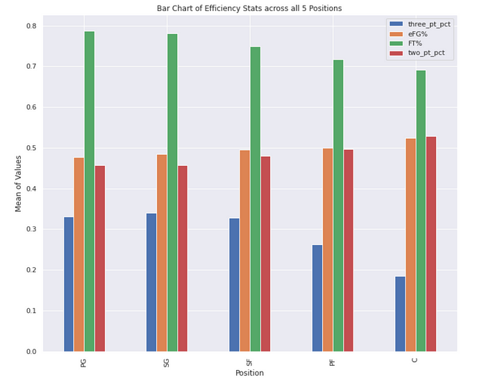
From the bar chart above, we can conclude that the maximum number of “Free Throw percentage” (FT%) is taken from the Point Guard (PG) position with the minimum number observed from the Center. Also, we can see that the Centre position © has the minimum “three pointers” made but the maximum “Effective field goal percentage” (eFG%) and “Two point percentage” (two_pt_pct) among all the positions. The highest efficiency of Center position could be explained by the fact that Center players dunk more often than shoot the ball, which is much more efficient and easy to make. Thus, the shots from the Center position are more accurate, which improves their “Effective field goal percentage” (eFG%). The least “Effective field goal percentage” (eFG%) and “Two point percentage” (two_pt_pct) are observed in the Point Guard (PG) and Shooting Guard (SG) positions.
#Seaborn Plot
import seaborn as sns
sns_df = df[['PTS/G', 'TRB/G', 'AST/G', 'STL/G', 'BLK/G', 'Height', 'WEIGHT','Pos']].head(300)
sns_df = sns_df.reset_index()
sns_df = sns_df.drop('index', axis=1)
sns_plot = sns.pairplot(sns_df, hue='Pos', size=2)
sns_plot

The Seaborn pair plot shows scatter plots of all possible x/y-axis combinations. The colors represent the different player positions. Diagonally, we see the distributions for each stat. For example, the points stat has similar distributions for all positions. However, defensive stats such as blocks and rebounds have a higher distribution for Centers, which are defensive positions.
Overall, most statistics have positive correlations. However, we must find a correlation when comparing offensive stats like assists and steals to defensive stats like blocks and rebounds. We can see where particular positions shine, such as Centers and their representation in the block and rebound charts, Point Guards, and the assist and teal charts.
We also see a positive correlation between a player's physical characteristics, which is expected; taller players tend to be heavier. The distributions for physical characteristics also match what we expect for each position. Centers are the tallest and heaviest, while Point Guards are the shortest and the lightest. Height and weight have a very positive correlation with blocking and rebounds.
A correlation matrix is used to see which features in the dataset are highly correlated.
correlation_mat = df.corr()
plt.rcParams['figure.figsize'] = (30, 20)
sns.heatmap(correlation_mat, annot = True )
plt.title("Correlation matrix ")
plt.xlabel("Player traits")
plt.ylabel("Player traits")

- Drop features that have correlation scores above 0.8 and have a high correlation with multiple features

- We ended up with traits that had lower correlation coefficients
- We included one trait, PF (Personal Fouls), as we hypothesized that Centers in a defensive position would have the most fouls (the results did not show this to be confirmed)
Question 1
Using classification models (Logistic Regression, Classification Trees, Random Forest, Gradient Boosted Trees), can we apply NBA player's weights and heights to classify players based on positions?
Logistic Regression
The probability of classification problems with two possible outcomes is modeled using logistic regression. The logistic function compresses the output of a linear equation between 0 and 1. It is used to predict the likelihood of a categorical dependent variable. The dependent variable in logistic regression is a binary variable that comprises data coded as 1 and 0. In other words, the logistic regression model predicts P(Y=1) as a function of X.
Stratified sampling is used since there is an imbalance in classes, and the preferred scoring metric is accuracy.
y=df_physical["Position"]
y=y.to_numpy()
X= df_physical[["Height","WEIGHT"]]
train_columns= X.columns
X=X.to_numpy()
X_tr, X_te, y_tr, y_te = train_test_split(X, y, test_size=0.2,stratify=y, random_state=42)
U_tr, U_val, v_tr, v_val = train_test_split(X_tr, y_tr, test_size=0.2,stratify=y_tr,random_state=42)
model = LogisticRegression(max_iter=10000)
model.fit(U_tr, v_tr)
y_pred = model.predict(U_val)
acc = accuracy_score(v_val, y_pred)
print(acc)
The accuracy on the validation set with Logistic Regression with one degree is 75.65%. Let’s see if we can increase the accuracy with Polynomial Features.
Polynomial Regression
Polynomial regression is a type of linear regression in which the data is fitted with a polynomial equation with a curved relationship between the target and independent variables. We use the sklearn PolynomialFeatures function to convert our data into a polynomial and then use linear regression to fit the parameters.
degrees = np.arange(1,5)

n_repeats = 100
accs_val = np.zeros((n_repeats, len(degrees)))

for i in range(n_repeats):
 U_tr, U_val, v_tr, v_val = train_test_split(X_tr, y_tr, test_size=0.2,stratify=y_tr, random_state= 2)
 for j, degree in enumerate(degrees):
 model = make_pipeline(StandardScaler(), PolynomialFeatures(degree=degree), LogisticRegression(max_iter=1000000))
 model.fit(U_tr, v_tr)
 accs_val[i, j] = accuracy_score(v_val, model.predict(U_val))

scores = accs_val.mean(axis=0)
degree = degrees[np.argmax(scores)]
ic(scores)
Result: array([0.74782609, 0.73913043, 0.72173913, 0.73043478])
There wasn’t an increase in accuracy scores after increasing the degrees. So, the underlying distribution is probably not polynomial.
model = LogisticRegression(max_iter=1000000)
model.fit(X_tr, y_tr)
y_pred = model.predict(X_te)
acc = accuracy_score(y_te, y_pred)
ic(acc)
So, the logistic regression accuracy on the test set is 67.36%.
dataframe_logistic=pd.DataFrame(model.coef_, columns=train_columns)
post_dict_reverse = {4:"C", 1:'PF', 0:'PG', 3:'SF', 2:'SG'}
dataframe_logistic=dataframe_logistic.reset_index()
dataframe_logistic.rename(columns = {'index':'position'}, inplace = True)
dataframe_logistic['position'] = dataframe_logistic.apply(lambda row: post_dict_reverse[row.position], axis=1)
dataframe_logistic.set_index("position")

From this, we can say that centers are taller and heavier than others, while Point Guards are shorter and weigh the least.
import seaborn as sns

from sklearn.metrics import confusion_matrix
cf_matrix=confusion_matrix(y_te, y_pred)
ax = sns.heatmap(cf_matrix, annot=True, cmap='Blues')
ax.set_title('Logistic Regression (Height and Weight) Confusion Matrix with labels\n\n');
ax.set_xlabel('\nPredicted Values')
ax.set_ylabel('Actual Values ');
#sns.set(rc = {'figure.figsize':(15,8)})
plt.rcParams['figure.figsize'] = (5, 5)
## Ticket labels - List must be in alphabetical order
ax.xaxis.set_ticklabels(list(dataframe_logistic["position"].values))
ax.yaxis.set_ticklabels(list(dataframe_logistic["position"].values))

## Display the visualization of the Confusion Matrix.
plt.show()
The confusion matrix is a helpful way to visualize the model’s accuracy. The correctly classified positions are on the left diagonal. For instance, we can see in the matrix that out of the 30 Point Guards included in the Testing Dataset, which is the sum of columns of the first row, the model correctly predicted Point Guard 20 times. 10 times, it thought the Point Guard was a Shooting Guard. It never thought the Point Guard was a Power Forward, and it never thought the Point Guard was a Center. That distribution makes sense — as the differing responsibilities of the positions increased, the model was less likely to predict that the Point Guard was in that position. The model finds it challenging to classify Power Forwards as the second row and misclassified it seven times as Small forward and six times as Center. The model predicts the best Center class, the fifth row, with only five instances of misclassification.
U, V, W = make_decision_regions(x=np.linspace(50,100, 200), y=np.linspace(150, 300, 200), model=model)
plt.figure(figsize=(5, 5))
ax = plt.gca()
ax.pcolormesh(U, V, W, shading="auto", alpha=0.1)
classes= list(dataframe_logistic['position'])
scatter=ax.scatter(*X_te.T, c=y_te)

legend1 = ax.legend(handles=scatter.legend_elements()[0],
 loc="lower left", title="Positions",labels=classes)
ax.add_artist(legend1)
plt.title("Logistic Regression (Height and Weight) Decision Regions")
plt.xlabel("Height (INCHES)")
plt.ylabel("Weight (LBS)")
plt.show()
plt.show()

Support Vector Classifier
GridSearchCV determines the ideal values for a particular model by tweaking the hyperparameter. It goes through the numerous parameters supplied into the parameter grid and finds the best combination depending on your preferred scoring metric (accuracy, f1, etc). GridSearchCV’s “best” parameters are theoretically the best that could be produced, but only by the parameters you included in your parameter grid.
C = [0.001, 0.01, 0.1, 1, 10, 100, 1000]
kernel = ["linear", "poly", "rbf", "sigmoid"]
search = GridSearchCV(SVC(), {"C": C, "kernel": kernel})
search.fit(X_tr, y_tr)
ic(search.best_params_)
model = search.best_estimator_
y_pred = model.predict(X_te)
acc_te = accuracy_score(y_te, y_pred)
ic(acc_te);
The best parameters are C= 0.1 and Kernel= Linear, with a testing accuracy of 66.7%
U, V, W = make_decision_regions(x=np.linspace(50,100, 200), y=np.linspace(150, 300, 200), model=model)
plt.figure(figsize=(5, 5))
ax = plt.gca()
ax.pcolormesh(U, V, W, shading="auto", alpha=0.1)
classes= list(dataframe_logistic['position'])
scatter=ax.scatter(*X_te.T, c=y_te)

legend1 = ax.legend(handles=scatter.legend_elements()[0],
 loc="lower left", title="Positions",labels=classes)
ax.add_artist(legend1)
plt.title("Support Vector Classifier(Height and Weight) Decision Regions")
plt.xlabel("Height (INCHES)")
plt.ylabel("Weight (LBS)")
plt.show()

import seaborn as sns

from sklearn.metrics import confusion_matrix
cf_matrix=confusion_matrix(y_te, y_pred)

ax = sns.heatmap(cf_matrix, annot=True, cmap='Blues')
ax.set_title('Support Vector Classifier (Height and Weight) Confusion Matrix with labels\n\n');
ax.set_xlabel('\nPredicted Values')
ax.set_ylabel('Actual Values ');
plt.rcParams['figure.figsize'] = (5, 5)
## Ticket labels - List must be in alphabetical order
ax.xaxis.set_ticklabels(list(dataframe_logistic["position"].values))
ax.yaxis.set_ticklabels(list(dataframe_logistic["position"].values))

## Display the visualization of the Confusion Matrix.
plt.show()

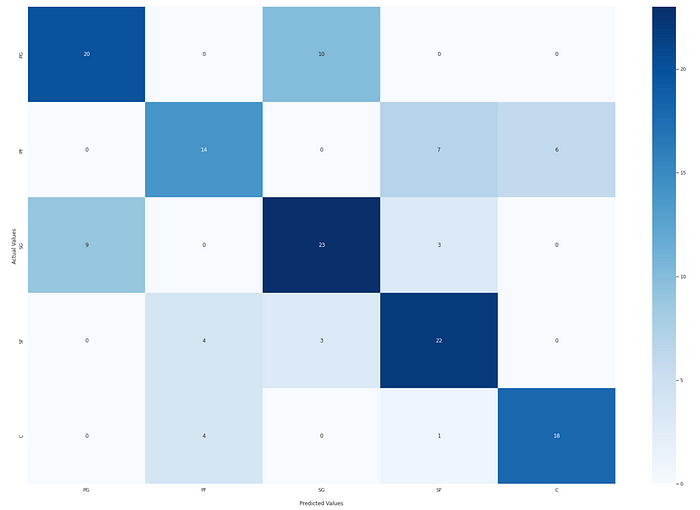
The Support Vector Classifier correctly predicts Point Guards for 21 out of 30 players in the test set, with it being incorrectly predicted as a Shooting Guard 9 times. Power Forwards are correctly predicted 14 out of 27 times, mispredicted as a Small Forward 7 times, and a Center 6 times. Shooting guards are identified correctly 22 out of 35 times; it is most misidentified as a Point Guard 10 times and as a Small Forward 3 times. Small Forwards are correctly identified 21 out of 29 times and misidentified as a Power Forward 5 times and a Shooting Guard 3 times. Centers are correctly identified 18 out of 23 times, misidentified as a power forward four times, and a Small Forward 1 time. Overall, these are reasonable, and when a player's position is misidentified, it is usually because the position they play has a height and weight overlap with other positions.
Decision Trees
Decision trees are supervised learning algorithms with a predefined target variable commonly utilized in non-linear decision-making with a primary linear decision surface. They can be adapted to solve classification or regression problems. The goal is to learn simple decision rules from data features to develop a model that predicts the value of a target variable. Different subsets of the dataset are formed due to the splitting, with each instance belonging to one of them. Terminal or leaf nodes are the final subsets, whereas internal or split nodes are the intermediate subsets. The average outcome of the training data in this node is used to predict the outcome in each leaf node.
Stratified sampling is used since there is an imbalance in classes, and the preferred scoring metric is accuracy.
from sklearn.tree import DecisionTreeClassifier
from sklearn import tree
U_tr, U_val, v_tr, v_val = train_test_split(X_tr, y_tr, test_size=0.2,stratify=y_tr,random_state=42)
max_depth = []
acc = []
acc_entropy = []
for i in range(1,30):
 dtree = DecisionTreeClassifier( max_depth=i)
 dtree.fit(U_tr, v_tr)
 pred = dtree.predict(U_val)
 acc.append(accuracy_score(v_val, pred))
 max_depth.append(i)

d = pd.DataFrame({'acc':pd.Series(acc),
 'max_depth':pd.Series(max_depth)})
# visualizing changes in parameters
plt.plot('max_depth','acc', data=d)
plt.xlabel('max_depth')
plt.ylabel('accuracy')
plt.legend()

A decision stump is a decision tree with only one node. The decision is entirely based on a single binary attribute of the sample.
A tree's maximum depth can be set to 5, as accuracy reaches a maximum at this level.
model = DecisionTreeClassifier(max_depth=5)
clf=model.fit(X_tr, y_tr)
#print(tree.plot_tree(clf))
y_pred=clf.predict(X_te)
acc_te = accuracy_score(y_te,y_pred )
ic(acc_te);
The accuracy obtained for the classification tree is 68.06%.
import seaborn as sns

from sklearn.metrics import confusion_matrix
cf_matrix=confusion_matrix(y_te, y_pred)

ax = sns.heatmap(cf_matrix, annot=True, cmap='Blues')
ax.set_title('Decision Tree Classifier (Height and Weight) Confusion Matrix with labels\n\n');
ax.set_xlabel('\nPredicted Values')
ax.set_ylabel('Actual Values ');
plt.rcParams['figure.figsize'] = (5, 5)
## Ticket labels - List must be in alphabetical order
ax.xaxis.set_ticklabels(list(dataframe_logistic["position"].values))
ax.yaxis.set_ticklabels(list(dataframe_logistic["position"].values))

## Display the visualization of the Confusion Matrix.
plt.show()

The Decision Tree Classifier for Height and Weight correctly predicts Point Guards for 23 out of 30 of the players in the test set, with it being incorrectly predicted as a Shooting Guard 7 times. Power Forwards are correctly predicted 11 out of 27 times, mispredicted as a Small Forward 4 times, and as a Center 12 times. This means it was more incorrectly predicted to be a Center than correctly identified as a power forward. Shooting guards are identified correctly 24 out of 35 times, it is most misidentified as a Point Guard 8 times, and as a Small Forward 3 times. Small Forwards are correctly identified 22 out of 29 times and misidentified as a Power Forward 3 times, a Shooting Guard 2 times, and a center two times. Centers are correctly identified 18 out of 23 times, misidentified as a power forward three times, and a Small Forward 2 times.
U, V, W = make_decision_regions(x=np.linspace(50,100, 200), y=np.linspace(150, 300, 200), model=model)
plt.figure(figsize=(5, 5))
ax = plt.gca()
ax.pcolormesh(U, V, W, shading="auto", alpha=0.1)
classes= list(dataframe_logistic['position'])
scatter=ax.scatter(*X_te.T, c=y_te)

legend1 = ax.legend(handles=scatter.legend_elements()[0],
 loc="lower left", title="Positions",labels=classes)
ax.add_artist(legend1)
plt.title("Decision Tree Classifier (Height and Weight) Decision Regions")
plt.xlabel("Height (INCHES)")
plt.ylabel("Weight (LBS)")
plt.show()

Random Forests
The Random Forest Classifier algorithm is an ensemble approach since it uses the Decision Tree Classifier method but creates several Decision Trees instead of just one. It takes advantage of random sampling, as each tree learns from a random sample of data points generated without replacement, and it only considers a subset of the features when splitting nodes. This randomization in the generation of individual trees reduces the risk of overfitting and increases the model’s overall predictive accuracy. This is because the final forecasts are calculated by averaging the results of each tree.
Compared to a single decision tree, the Random Forest Classifier allows us to investigate the importance of the feature more deeply. This is because, whereas a single decision tree may focus on a specific area of the data and connect high importance with that feature even if it doesn’t, random sampling and feature selection over numerous decision trees allow us to find which features consistently have high relevance. We can use the average predictive ability of the features to reduce the variance associated with feature importance if we use a single tree by generating many trees.
We can either eliminate features that aren’t important and re-run the models with this knowledge, or we can use the information to determine which features aren’t vital for the model. Removing features reduces the model’s complexity and, hence, the compute time, so the trade-off is between the information acquired from features and the compute time.
from sklearn.ensemble import RandomForestClassifier, AdaBoostClassifier
from sklearn.ensemble import GradientBoostingClassifier

n_estimators_grid = np.arange(1, 50)
gd_accs_te = []
rf_accs_te = []
U_tr, U_val, v_tr, v_val = train_test_split(X_tr, y_tr, test_size=0.2,stratify=y_tr,random_state=42)
for n_estimators in tqdm(n_estimators_grid):
 gbt1_model = make_pipeline(StandardScaler(), GradientBoostingClassifier(n_estimators=n_estimators, random_state=1))
 gbt1_model = gbt1_model.fit(U_tr, v_tr)
 gd_acc = accuracy_score(v_val, gbt1_model.predict(U_val))
 gd_accs_te.append(gd_acc)

 rf1_model = make_pipeline(StandardScaler(), RandomForestClassifier(n_estimators=n_estimators, random_state=42))
 rf1_model = rf1_model.fit(U_tr, v_tr)
 rf_acc = accuracy_score(v_val, rf1_model.predict(U_val))
 rf_accs_te.append(rf_acc)
plt.ylim(0.1, 1)
plt.xlabel("n_estimators", fontsize=12)
plt.ylabel("test accuracy", fontsize=12)
plt.title("Classifier Performance", fontsize=14)
plt.plot(n_estimators_grid, gd_accs_te, lw=3, label="GradientBoost")
plt.plot(n_estimators_grid, rf_accs_te, lw=3, label="Random Forest")
#plt.plot([0, 300], [mean_stump_acc, mean_stump_acc], "m--", lw=2, label="Stump baseline")
#plt.plot([0, 300], [mean_tree_acc, mean_tree_acc], "g--", lw=2, label="Tree baseline")
plt.legend(fontsize=12, loc="lower right")
plt.show()

ic (max(rf_accs_te),rf_accs_te.index(max(rf_accs_te)))
Result: (0.7304347826086957, 6)
ic (max(gd_accs_te),gd_accs_te.index(max(gd_accs_te)))
Result: (0.7304347826086957, 23)
We get maximum test accuracy with random forests when no_of_estimators = 6, around 73 percent; we get the same accuracy as a gradient-boosted tree with 23 estimators; we will build Random forests as they have fewer estimators.
rf1_model = make_pipeline(StandardScaler(), RandomForestClassifier(n_estimators=6, random_state=42))
rf1_model = rf1_model.fit(X_tr, y_tr)
y_pred = rf1_model.predict(X_te)
rf_acc = accuracy_score(y_te, y_pred)
rf_acc
The accuracy of the test dataset for random forests for the height and weight features is 69.4%.
from sklearn.inspection import permutation_importance

result = permutation_importance(rf1_model, X_te, y_te, n_repeats=10, random_state=1, n_jobs=2)
forest_importances = pd.Series(result.importances_mean, index=np.array(train_columns))
fig, ax = plt.subplots()
forest_importances.plot.bar(yerr=result.importances_std, ax=ax)
ax.set_title("Feature importances using permutation on full model")
ax.set_ylabel("Mean accuracy decrease")
fig.tight_layout()
plt.show()

import seaborn as sns

from sklearn.metrics import confusion_matrix
cf_matrix=confusion_matrix(y_te, y_pred)
ax = sns.heatmap(cf_matrix, annot=True, cmap='Blues')
ax.set_title('Random Forest (Height and Weight) Confusion Matrix with labels\n\n');
ax.set_xlabel('\nPredicted Values')
ax.set_ylabel('Actual Values ');
plt.rcParams['figure.figsize'] = (5, 5)
## Ticket labels - List must be in alphabetical order
ax.xaxis.set_ticklabels(list(dataframe_logistic["position"].values))
ax.yaxis.set_ticklabels(list(dataframe_logistic["position"].values))

## Display the visualization of the Confusion Matrix.
plt.show()

The Random Forest Classifier for Height and Weight correctly predicts Point Guards for 24 out of 30 of the players in the test set, with it being incorrectly predicted as a Shooting Guard 6 times. Power Forwards are correctly predicted 20 out of 27 times, mispredicted as a Small Forward 4 times, and as a Center 3 times. For Height and Weight Classification, the Random Forest classifier accurately classifies Power Forwards. Shooting guards are identified correctly 22 out of 35 times; it is most misidentified as a Point Guard 9 times and as a Small Forward 4 times. Small Forwards are correctly identified 19 out of 29 times and misidentified as a Power Forward 4 times, a Shooting Guard 4 times, and a center two times. Centers are correctly identified 15 out of 23 times; it is misidentified as a Power Forward 6 times and a Small Forward 2 times.
U, V, W = make_decision_regions(x=np.linspace(50,100, 200), y=np.linspace(150, 300, 200), model=model)
plt.figure(figsize=(5, 5))
ax = plt.gca()
ax.pcolormesh(U, V, W, shading="auto", alpha=0.1)
classes= list(dataframe_logistic['position'])
scatter=ax.scatter(*X_te.T, c=y_te)

legend1 = ax.legend(handles=scatter.legend_elements()[0],
 loc="lower left", title="Positions",labels=classes)
ax.add_artist(legend1)
plt.title("Random Forest (Height and Weight) Decision Regions")
plt.xlabel("Height (INCHES)")
plt.ylabel("Weight (LBS)")
plt.show()

KNN classification
The K-NN method assumes that the new case/data and existing cases are similar and places the latest case in the most similar category to the existing categories. The KNN method stores all available data and classifies a new data point based on its similarity to the existing data. This means new data can be quickly sorted into categories using the KNN method.
ks = np.arange(1, 50, 2)

n_repeats = 200
accs_val = np.zeros((n_repeats, len(ks)))

for i in tqdm(range(n_repeats)):
 U_tr, U_val, v_tr, v_val = train_test_split(X_tr, y_tr, test_size=0.2,stratify=y_tr)
 for j, k in enumerate(ks):
 model = KNeighborsClassifier(n_neighbors=k)
 model.fit(U_tr, v_tr)
 accs_val[i, j] = accuracy_score(v_val, model.predict(U_val))

scores = accs_val.mean(axis=0)
k = ks[np.argmax(scores)]
ic(k)
The best number of neighbors is 11.
plt.plot(ks, scores)
plt.vlines(k, *plt.ylim(), colors="k", linestyles=":", label=f"max. validation accuracy,
={k}")

model = KNeighborsClassifier(n_neighbors=k)
model.fit(X_tr, y_tr)
y_pred=model.predict(X_te)
acc_knearest= accuracy_score(y_pred,y_te)
print(acc_knearest)
The accuracy of the test dataset for random forests for the features' height and weight is 65.3%.
import seaborn as sns

from sklearn.metrics import confusion_matrix
cf_matrix=confusion_matrix(y_te, y_pred)
ax = sns.heatmap(cf_matrix, annot=True, cmap='Blues')
ax.set_title('KNN classification (Height and Weight) Confusion Matrix with labels\n\n');
ax.set_xlabel('\nPredicted Values')
ax.set_ylabel('Actual Values ');
plt.rcParams['figure.figsize'] = (5, 5)
## Ticket labels - List must be in alphabetical order
ax.xaxis.set_ticklabels(list(dataframe_logistic["position"].values))
ax.yaxis.set_ticklabels(list(dataframe_logistic["position"].values))

## Display the visualization of the Confusion Matrix.
plt.show()

The KNN Classifier for Height and Weight correctly predicts Point Guards for 22 out of 30 players in the test set, with it being incorrectly predicted as a Shooting Guard 8 times. Power Forwards are correctly predicted 16 out of 27 times, mispredicted as a Small Forward 5 times, a Center 5 times, and a Shooting Guard 1 time. Shooting guards are identified correctly 21 out of 35 times; it is most misidentified as a Point Guard 10 times and as a Small Forward 4 times. Small Forwards are correctly identified 20 out of 29 times and misidentified as a Power Forward 6 times and a Shooting Guard 3 times. Centers are correctly identified 15 out of 23 times; it is misidentified as a Power Forward 7 times and a Small Forward 1 time.
U, V, W = make_decision_regions(x=np.linspace(50,100, 200), y=np.linspace(150, 300, 200), model=model)
plt.figure(figsize=(5, 5))
ax = plt.gca()
ax.pcolormesh(U, V, W, shading="auto", alpha=0.1)
classes= list(dataframe_logistic['position'])
scatter=ax.scatter(*X_te.T, c=y_te)

legend1 = ax.legend(handles=scatter.legend_elements()[0],
 loc="lower left", title="Positions",labels=classes)
ax.add_artist(legend1)
plt.title("KNN Classifier (Height and Weight) Decision Regions")
plt.xlabel("Height (INCHES)")
plt.ylabel("Weight (LBS)")
plt.show()

Most of the classifiers we used predicted positions reasonably when using Height and Weight. Even when the classifiers incorrectly predicted a position, it was usually sensible. For example, defensive positions were misclassified as other defensive positions, or positions mainly made up by big men were predicted as other positions made up by large men.
The next blog will use PCA and K Means clustering to discover the most productive players and seasons by position. I’d love to hear any thoughts, comments, or questions about the Moneyball for NBA series. Feel free to reach out at my website or LinkedIn.
References
Data Sources
- ‘NBA Player Stats — Dataset by Etocco’. Data.World, https://data.world/etocco/nba-player-stats.
Other Sources
- D’Angelo, John. Research Guides @ Fordham: Copyright Resources: Creative Commons & Public Domain. https://fordham.libguides.com/copyright/Licensing.
- Wilkinson, P. (2021, October 29). Introduction to random forest classifiers. Medium. Retrieved from https://towardsdatascience.com/introduction-to-random-forest-classifiers-9a3b8d8d3fa7
- Fischler, B. (2021, February 9). NBA Machine Learning Position Predictor. Medium. Retrieved from https://medium.com/analytics-vidhya/nba-machine-learning-position-predictor-488fef42ac1c
- G. L. T.(2022, March 22). Hyperparameter tuning with GRIDSEARCHCV. GreatLearning Blog: Free Resources what Matters to shape your Career! Retrieved from https://www.mygreatlearning.com/blog/gridsearchcv/
- Molnar, C. (2022, March 29). Interpretable machine learning. 5.4 Decision Tree. Retrieved from https://christophm.github.io/interpretable-ml-book/tree.html
- ‘Polynomial Regression | Polynomial Regression In Python’. Analytics Vidhya, 15 Mar. 2020, https://www.analyticsvidhya.com/blog/2020/03/polynomial-regression-python/.
- Yadav, Ajay. ‘DECISION TREES’. Medium, 11 Jan. 2019, https://towardsdatascience.com/decision-trees-d07e0f420175.
- ‘Regex — Changing Height (Feet and Inches) to an Integer in Python Pandas’. Stack Overflow, https://stackoverflow.com/questions/26986655/changing-height-feet-and-inches-to-an-integer-in-python-pandas.
- Variance Inflation Factor (VIF) Explained — Python. https://etav.github.io/python/vif_factor_python.html.
- Scatter Plots — Problem Solving with Python. https://problemsolvingwithpython.com/06-Plotting-with-Matplotlib/06.10-Scatter-Plots/.
- Matplotlib.Axes.Axes.Scatter — Matplotlib 3.5.0 Documentation. https://matplotlib.org/3.5.0/api/_as_gen/matplotlib.axes.Axes.scatter.html.
- ‘Feature Importances with a Forest of Trees’. Scikit-Learn, https://scikit-learn/stable/auto_examples/ensemble/plot_forest_importances.html.
- Lee, Ceshine. ‘Feature Importance Measures for Tree Models — Part I’. Veritable, 8 Sept. 2020, https://medium.com/the-artificial-impostor/feature-importance-measures-for-tree-models-part-i-47f187c1a2c3.
- ‘R — How to Interpret Mean Decrease in Accuracy and Mean Decrease GINI in Random Forest Models’. Cross Validated, https://stats.stackexchange.com/questions/197827/how-to-interpret-mean-decrease-in-accuracy-and-mean-decrease-gini-in-random-fore.
- ‘Python — How to Fix the Values Displayed in a Confusion Matrix in Exponential Form to Normal Form’. Stack Overflow, https://stackoverflow.com/questions/61748441/how-to-fix-the-values-displayed-in-a-confusion-matrix-in-exponential-form-to-nor.
- Wilkinson, Philip. ‘Introduction to Random Forest Classifiers’. Medium, 29 Oct. 2021, https://towardsdatascience.com/introduction-to-random-forest-classifiers-9a3b8d8d3fa7.
Join thousands of data leaders on the AI newsletter. Join over 80,000 subscribers and keep up to date with the latest developments in AI. From research to projects and ideas. If you are building an AI startup, an AI-related product, or a service, we invite you to consider becoming a sponsor.
Published via Towards AI
Related posts
Popular posts

 for 2021")


Updates

Recent Posts

