


")
Backpropagation and Vanishing Gradient Problem in RNN (part 1)
Last Updated on July 26, 2023 by Editorial Team
Author(s): Alexey Kravets
Originally published on Towards AI.
Theory and code
Introduction
In this article, I am not going to explain the applications or intuition about the RNN model — indeed, I expect the reader to already have some familiarity with it, together with the vanishing gradient problem and general backpropagation algorithm. I will also show where the vanishing gradient problem comes from during backpropagation highlighting some details which are often misunderstood.
I will cover a many-to-many architecture of Recurrent Neural Network, which means that we have, for example, a sequence of characters as input, and we want the model to be able to predict the next following characters for the next T timesteps.
Forward propagation
Let’s first look at how forward propagation through time is performed. For simplicity, we assume to have 3 timesteps. RNN with 3 timesteps would look like below :
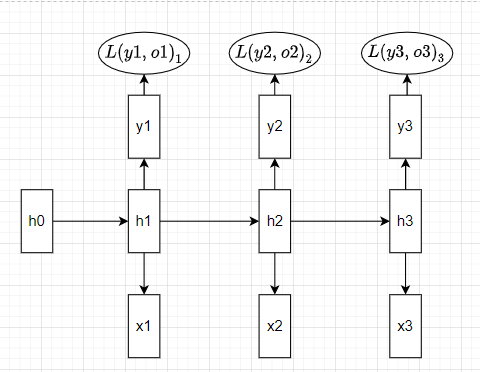
And formulas of different components:

Thus we have, input Xₜ of shape (N — number of examples, T —timesteps, i.e., number of characters or words, D — embedding dimension), hidden state vector hₜ that stores the information about the past of shape (N, H — hidden dimension), Wₕₕ — weight matrix for hₜ of shape (H, H), Wₓₕ — weight matrix for Xₜ of shape (D, H) and weight matrix Wᵧₕ to predict the output yₜ of shape (H, V — vocabulary length). Starting from the input and previous hidden state, we get the next hidden state hₜ and the output predicted for that state yₜ. Notice that RNN uses the same weights matrices for each time step instead of learning different matrices at different timesteps, which would require a lot of memory and would be inefficient given that we often end up with models with a very high number of timesteps.
Backpropagation
Backpropagation through time is a bit more tricky than normal backpropagation in feed-forward neural networks, as the parameters for different timesteps are shared, and also hidden state in the next layer depends on the hidden states from the previous layers.
Looking at the forward propagation formulas (figure 2) above, let’s compute the partial derivatives with respect to different elements:

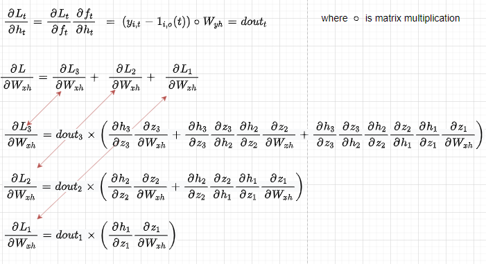
Let’s compute the derivative of all the individual losses at each timestep with respect to Wₓₕ (the other parameters can be computed analogously) as all the losses are modified by weights parameters. First of all, notice how Wₓₕ affects the outputs through the current hidden state but also through previous hidden states that all depend on Wₓₕ (red arrows). So computing the partial derivative of L2 with respect to h2 becomes as in figure 4 below.

Let’s now look at the total Loss, which is the sum of all the single losses. We can notice that when computing the derivative of total L with respect to h2 we have 2 components or directions (red arrows) at h2 — the first coming from L3 through h3 and the second from L2.

Now let’s compute the derivative of Wₓₕ with respect to the total Loss, which is the sum of all the single losses:
When coding the backpropagation, we compute these derivatives in a loop :
At first sight, it might look different from the solution in figure 6. Thus, for a better understanding, let’s analyze and expand on what is happening in the code (notice that we sum the partial derivatives in red squared to compute the total derivative of Wₓₕ) :

Now it should be more clear that the code and the results in figure 6 are exactly the same.
Vanishing gradients
It is well known that RNNs suffer from vanishing gradients, which happens because many Wₕₕ matrices that are the result of the partial derivative of h with respect to z (figure 6) are multiplied together, provoking the gradient to vanish if the Largest singular value of Wₕₕ is < 1 or to explode if > 1 (here we assume the first case). However, this concept is often misinterpreted, thinking that the entire gradient of some coefficients does vanish.
In reality, the derivative of total Loss with respect to Wₓₕ does not become zero, but the gradients of a particular loss Li with respect to Wₓₕ will be zero for inputs further away from Li which will not be considered when adjusting the weights Wₓₕ but might be more important than the local context to predict yi correctly.
For example, when doing backpropagation with respect to L3, which is affected by all the previous timesteps, to reduce that particular loss it will highly rely on the gradients coming from the closest timesteps where the products are between a few terms, and thus trying to adjust the weights considering mainly inputs Xₜ closer to L3 and ignoring inputs further away because the information (gradients) from those timesteps are zero due to multiplication of more terms that tend to vanish.

And so, the last term in the red square (contains the context about how X₁ affects L3) will be close to zero, while the first two terms in the blue square (contain the context about how X₂ and X₃ affect L3) will not be close to zero, and this information will be then used to adjust the weights Wₓₕ trying to reduce L3.
For clarification, if we assume a sentence of 6 words: “Because no food was available in the market, John had to skip dinner.” In this case, to predict the word “dinner” the model needs to refer to “food”. But because the gradient of the Loss for word “dinner” wrt Wₓₕ will be close to zero for the part of the sum related to word “food”, it will not be taken into account in Wₓₕ and the model will try to adjust this weight mainly relying on words close to “dinner” which provide almost no relevant information to predict “dinner”.
Numerical Example
In the code below, we compute gradients for all Xᵢ components of each Loss wrt Wₓₕ . For example, losses[2] contain the gradients of how X₁, X₂, and X₃ affect L3, as shown in figure 8. This way, we can then see the effect of the vanishing gradient numerically.
Let’s see the gradients for the Loss L3 for each component:
display(losses[2])

{0: array([[ 0.0132282 , 0.01965245, 0.00556892, -0.01311703],
 [-0.00498197, -0.00740145, -0.00209735, 0.0049401 ],
 [-0.00430128, -0.00639019, -0.00181079, 0.00426513]]),
 1: array([[ 0.00375982, 0.01506674, 0.01860143, 0.00016598],
 [-0.0030325 , -0.01215215, -0.01500307, -0.00013388],
 [ 0.0080649 , 0.03231846, 0.03990044, 0.00035604]]),
 2: array([[-0.12964021, -0.36447594, 1.01880983, 0.68256384],
 [ 0.05655798, 0.15900947, -0.44447492, -0.2977813 ],
 [-0.02370473, -0.06664448, 0.18628953, 0.1248069 ]])}

display([f"component {e+1} : {np.linalg.norm(losses[2][e])}" for e in losses[2]])

# Let's see the magnitudes of them:

['component 1: 0.03087853793900866',
 'component 2: 0.06058764108583098',
 'component 3: 1.4225029296044476']
From the above, we can see that X₃ , which is the closest to L3 has the largest update, while X₁ and X₂ contribute much less to Wₓₕ update.
We can also see that, as in figure 8, the sum of the gradients of all losses across all components is equal to the total gradient dWx.
# we can also see that if we sum all the losses across all
# components we get total gradient for dWx
np.allclose(dWx, np.sum([losses[l][e] for l in losses for e in losses[l]], 0))
# Output : True
Conclusions
Obviously, you don’t need to do backpropagation yourself in reality, as many software abstract out all the maths of backpropagation. It is a good exercise, though, to do all the derivations by hand to understand these models better. That’s why you should now try to do the same for other parameters — Wₕₕ, Wᵧₕ, b, and Xₜ.
References
http://cs231n.stanford.edu/
https://jramapuram.github.io/ramblings/rnn-backrpop/
https://ieeexplore.ieee.org/document/279181/
Join thousands of data leaders on the AI newsletter. Join over 80,000 subscribers and keep up to date with the latest developments in AI. From research to projects and ideas. If you are building an AI startup, an AI-related product, or a service, we invite you to consider becoming a sponsor.
Published via Towards AI
Related posts


Popular posts

 for 2021")


Updates

Recent Posts


