Univariate Linear Regression From Scratch

Author(s): Erkan Hatipoğlu

Originally published on Towards AI the World’s Leading AI and Technology News and Media Company. If you are building an AI-related product or service, we invite you to consider becoming an AI sponsor. At Towards AI, we help scale AI and technology startups. Let us help you unleash your technology to the masses.

With Code in Python

Introduction

Generally, one of the first subjects of a Machine Learning Course is Linear Regression, which is not very complex and easy to understand. Moreover, it includes many Machine Learning notions that can be used later in more complex concepts. So it is reasonable to start with Linear Regression to a new Machine Learning basics series.

In this blog post, we will learn about Univariate Linear Regression which means Linear Regression with just one variable. At the end of this article, we will understand fundamental Machine Learning concepts such as the hypothesis, cost function, and gradient descent. In addition, we will write the necessary code for those functions and train/test a linear model for a Kaggle dataset using Python [1].

Before diving into Univariate Linear Regression, let's briefly talk about some basic concepts:

Basic Concepts

Machine Learning is the subfield of Artificial Intelligence that uses data to program computers for some tasks. A typical Machine Learning application uses a dataset and a learning algorithm to make a model that can then predict the outputs for new inputs to the application.

Machine Learning applications are generally divided into three categories:

• Supervised Learning
• Unsupervised Learning
• Reinforcement Learning

In supervised learning [2], the data have identical features that can be mapped to some label. Supervised learning has two types.

It is called classification if the number of labels is limited and can be transformed into some categories. Identifying animals or handwritten digits in images are examples of classification.

If the set of labels is not restricted to some small number of elements but can be assumed infinitely many, then it is called regression. Predicting the price of houses in a region or gas usage per kilometer of cars are regression examples.

In unsupervised learning [3], the dataset has no labeled data. After the teaching process, the model discovers the patterns in the data. Categorizing the customers of an e-commerce website is an example of unsupervised learning.

Reinforcement learning [4] uses intelligent agents who act according to reward and punishment mechanisms [5]. It is mainly used in computer gaming.

Linear Regression

As we have said above, regression maps inputs to infinitely many outputs. In addition, Linear Regression suggests a linear relationship between the inputs and outcomes [6]; it is challenging to visualize this if we have more than one input variable. If we have one input variable, we need to draw a line in the XY plane; if we have two input variables, we need to construct a plane in the three-dimensional coordinate system. More than two input variables are extremely tough to imagine. As a result, we will demonstrate Linear regression using univariate data. Below are the housing prices from Portland, Oregon dataset [7], which we will use as an example.

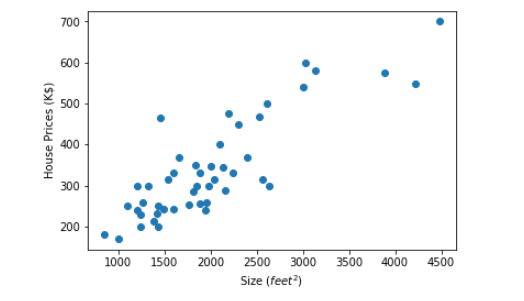
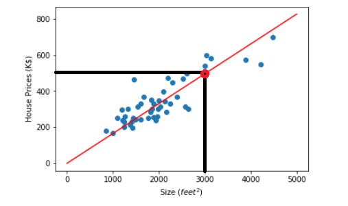
In the graph above, the y-axis is the price (K$) of some houses in Portland, and the x-axis is the house's size (feet²). We want to draw a straight line on this graph (such as the image below) so that when we know the size of a new home not in this dataset, we can predict its price by using that line.

For example, we can predict that the price of a 3000 feet² house is approximately 500 K$, as seen in the graph below.

So without further ado, let's dive into more profound concepts to understand how to draw that line.

Note that this article uses the Linear Regression dataset [1] and Univariate Linear Regression from Scratch notebook [8] from Kaggle. As described in the content part of the dataset, it has a training dataset of 700 and a test dataset of 300 elements. The data consists of pairs of (x,y) where x’s are numbers between 0 and 100 and y’s have been generated using the Excel function NORMINV(RAND(), x, 3). It is also given that the best estimate for y should be x.

First, we must write three functions to find a univariate linear regression solution on a dataset. These functions are for the hypothesis, cost, and gradient descent calculations in order. Foremost, we will explain them one by one.

The Hypothesis

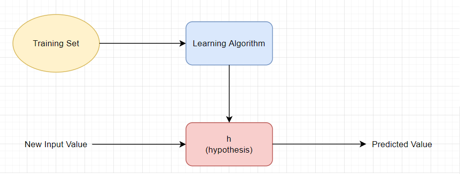
We aim to find a model we can use to predict new inputs. A hypothesis is a potential model for a machine learning system [9].

As seen in the figure below, we can find the hypothesis for a dataset by using a learning algorithm [10]. Later we will talk about how well this hypothesis fits our data but for now, let's just define the hypothesis formula.

For a univariate linear regression task, the hypothesis is of the form:

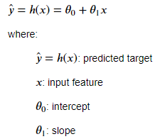
The intersection of the y-axis with the hypothesis line is called intercept. This is θ₀ in our formula, and the slope of the hypothesis line is θ₁.

If we know x, θ₀, and θ₁ values, we can predict the target value for a machine learning system. For example, in the housing prices example above, θ₀ = 0.00008, and θ₁ = 0.16538 for the red line. So for a house of 3000 feet² (x=3000), the expected price is:

As can be seen, we need three parameters to write the hypothesis function. These are x (input), θ₀, and θ₁. So, let's write the Python function for the hypothesis:

https://medium.com/media/3c752accc7341b367a1a05bcd7148652/href

The process is pretty straightforward. We just need to return (θ₀+ θ₁* x).

The Cost Function

When we have a hypothesis (i.e., we know the values of θ₀ and θ₁), we must decide how well this hypothesis fits our data. Turning back to the housing prices example, Let's take θ₀ as 500 and θ₁ as -0.1 and draw the line on our data.

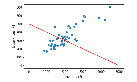
As seen from the image above, A hypothesis with θ₀ = 500 and θ₁ = -0.1 is not a good match for our dataset. We do not want such a hypothesis to be our model since it gives faulty results except for a few points. Let's draw some more lines to have a better understanding.

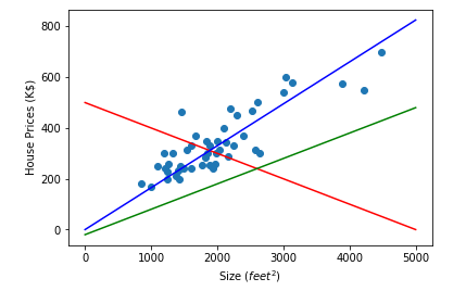
We have three hypotheses in the above image with different θ values. By intuition, we can easily pick the blue line (θ₀ = 0, θ₁ = 0.165) as the best match for our data. The question is, how can we select a better fit mathematically? In other words, how can we choose the best θ₀ and θ₁ values that give the optimum solution to our goal of finding a model we can use to predict new inputs?

To do that, we can choose θ₀ and θ₁ such that h(x) is close to the actual value for all training examples [10]. We make errors for each point on the dataset for a specific hypothesis (with known θ₀ and θ₁ values). If we somehow add all of those errors we made for each data point on that dataset, we can choose the best fitting line by selecting the minimum sum (which means we make fewer errors).

So we define a cost function to measure the total error we make. There are several solutions we can choose. One is called the squared error function:

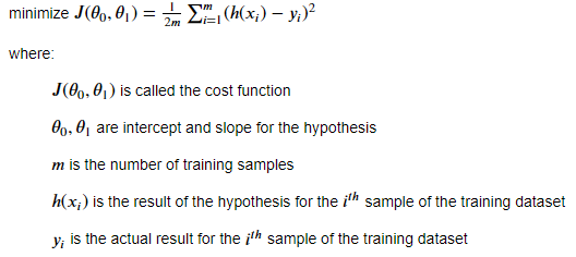
j(θ₀, θ₁) is called the cost function. It is a function of θ₀ and θ₁, which are the intercept and slope of the hypothesis. h(xᵢ) — y(xᵢ) is the error we made for the ith training example. And by squaring it, we get two significant benefits; first, we punish big mistakes, and second, we get rid of the negative sign if h(x) < y. By dividing the total sum of errors by the number of samples, we find the average error we made. As described above, smaller cost function values suggest a better match, so we are trying to minimize the cost function for a better fit.

To write the cost function, we must import NumPy, a famous machine learning library used for linear algebra tasks. NumPy will speed up our calculations. We also need four parameters, and these are θ₀, θ₁, X (input), and y (actual output).

https://medium.com/media/35573f7a65979d23a099699df08bd009/href

Inside the function, the first thing to do is to calculate the errors for each data point using NumPy's subtract function. Then we can calculate the square errors for each data point using NumPy's square function. Finally, we can calculate the total square error using sum() and divide by the number of examples to get the average error. Note that all the training data is passed to the function as a NumPy array. In addition, since we are using the hypothesis function inside the cost function, we must write it prior. Remember also that we are not trying to minimize the cost function yet. We will see how to do it later in the Gradient Descent topic.

Gradient Descent

Now we can calculate the cost function for a given set of θ₀ and θ₁ on a dataset. We also know that the θ₀ and θ₁ values that make the cost function minimum are the best matches for our data. The next question is how to find those θ₀ and θ₁ values that make the cost function minimum.

The gradient descent algorithm can be utilized for this purpose, and we can use the climber analogy to explain gradient descent better. Suppose there is a climber at the top of a mountain. He wants to descend to the hillside as soon as possible. So, he observes his surroundings and finds the steepest path to the ground, moving one tiny step in that direction. Then he observes his surroundings again to see the new, most vertical direction to move. He keeps going repeating this procedure till he reaches the hillside.

The explanation is beyond this blog post, but we know that the squared error cost function has one global minimum with no local minimums. Furthermore, its negative gradient at a point is the steepest direction to this global minimum. So like a climber on the top of a mountain finds his way to the hillside, we can use gradient descent to find the θ values that minimize our cost function.

To do that, first, we need to select some initial θ₀ and θ₁ to start with. Then, we can calculate the gradient descent at this point and change θ₀ and θ₁ values proportional to the negative gradient calculated. Then repeat the same steps till convergence.

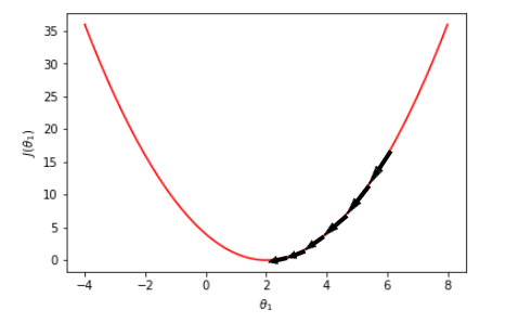
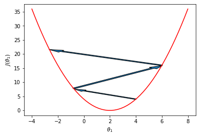
To better understand the concept of gradient, we will use a random squared error cost function with θ₀ = 0, as shown below. We select θ₀ as zero; otherwise, we would have struggled with a 3D graph instead of dealing with a 2D one.

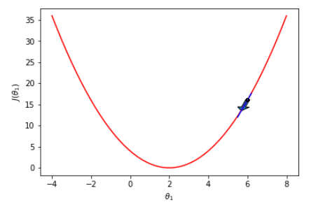
In the image above, suppose we are at point = 6 (that is, we have selected our initial θ₁ as 6) and trying to reach the global minimum. The negative gradient at this point is downward, as shown by the arrow. So if we go one step further in that direction, we will end with a point smaller than 6. Then, as shown below, we can repeat the same procedure till convergence at point = 2.

Let's try another point as below. If we have selected another θ₁ value, such as point = -2, the negative gradient at this point would be downward, as shown by the arrow. So if we go one step further in that direction, we will end with a value larger than -2.

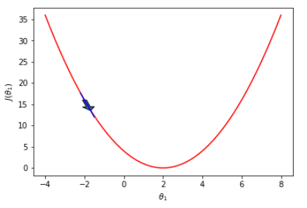
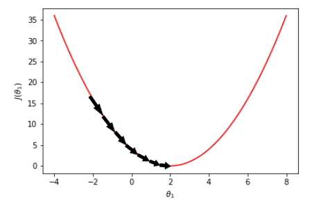
Then, as shown below, we can repeat the same procedure till convergence at point = 2.

One good question to ask is how to decide when we have converged. That is, what is our stop condition at the code? We have two choices. We can either check the value of the cost function and stop if it is smaller or equal to a predefined value, or we can check the difference between consecutive cost function values and stop if it is smaller or equal to a threshold value. We will choose the latter since, due to the initial θ values selection, we can never reach the predefined cost value we have selected.

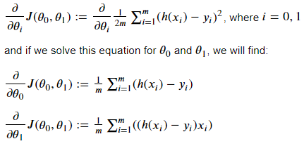
Taking the gradient descent of a function is a freshman-level Calculus concept, and we will not dive into details; instead, we will only give the outcomes. The gradient of the squared error cost function for a univariate dataset is as follows:

Before writing the code for the gradient descent, we must introduce one final concept: the learning rate. As we have discussed above, the gradient descent algorithm requires tiny steps, and as shown below, we may risk overshooting the local minimum if the steps are too big. So, while calculating the new θ values, we multiply the gradient result with the learning rate coefficient. The learning rate is a hyperparameter that needs to be adjusted during training. While a higher learning rate value may result in overshooting, a smaller learning rate value may result in higher training time [10].

As a result, for a univariate dataset with a hypothesis of the form h(x) = θ₀ + θ₁* x and a squared error cost function J(θ₀, θ₁), the θ values for each step can be calculated as follows:

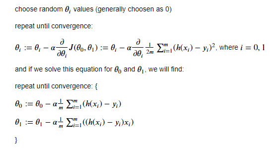
As discussed, α is the learning rate, and m is the number of training examples.

To write the gradient descent function, we must import NumPy as in the cost function. We also need five parameters, and these are θ₀, θ₁, α (learning rate), X (input), and y(actual output). We also must be sure not to update θ₀ before calculating θ₁ [10]. Otherwise, we will end up with a faulty result. The code for the gradient function is as follows:

https://medium.com/media/056fef8e039afb98be49d187a0bb6688/href

Inside the function, the first thing to do is to calculate the errors for each data point using NumPy's subtract function and store it in a variable. Then we can multiply the previous result with x and store it in another variable. Note that all the training data is passed to the function as a NumPy array. So those variables are of type array, and the sum() function can be used to get the total values which then can be multiplied by the learning rate and divided by the number of examples. As a final step, we can calculate and return the new θ values.

Model Training

Since we have written all the functions we need, it is time to train the model. As discussed before, we need to decide when the gradient descent converges. To do that, we will subtract consecutive cost values. If the difference is smaller than a certain threshold, we will conclude that the gradient descent converges.

We also draw the hypothesis for each iteration to see how it changes. But this slows down the code. The selection of initial values may significantly change the number of iterations, so it may be suitable to change this part of the code for those who reproduce it. It is also possible to copy the Univariate Linear Regression from Scratch notebook for this purpose, in which a section draws the model trained only because of high iteration counts.

https://medium.com/media/dd9d0e42e37b49b18522ffb487115f1f/href

Inside the code block, we first initialize the α, θ₀, θ₁, and the convergence threshold values. We also calculate the initial cost value by calling the cost function.

As previously discussed, our stop condition for the while loop is the difference of consecutive cost function values to be smaller than a threshold value. We first draw the training data and the hypothesis for demonstration purposes for each while loop iteration. We then calculate the cost function value by calling the cost function. Next, we calculate the new θ₀ and θ₁ values by calling the gradient function. Next, we use new θ values to recalculate the cost value to find the difference to check the stop condition. At the end of the loop, we print some necessary information for each iteration.

The Result

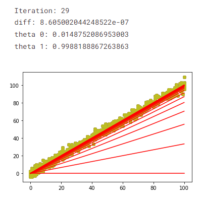
The result below is for the initial conditions in the model training code block. The training took 29 iterations. θ₀ is calculated at approximately 0.015, and θ₁ is around 0.999. The final cost value is calculated as about 15.742. The result is very close to the y = x line discussed in the Linear Regression Dataset. We can also see the change in the hypothesis for each iteration.

Validation

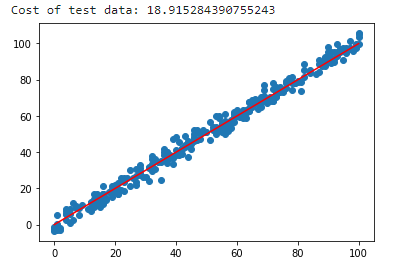
We can also validate our result with the test dataset, which hasn't been used in the training process. Below you can find the performance of our model concerning the test dataset. The cost value of the model is approximately 18.915, slightly worse than 15.742 (training cost value), which is expected.

Conclusion

In this blog post, we learned the basics of linear regression, such as the hypothesis, the cost function, and the gradient descent using univariate data. We also wrote those functions in Python. In addition, using them, we have trained a univariate linear model and tested it utilizing the Linear Regression dataset.

Interested readers can find the code used in this blog post in the Kaggle notebook Univariate Linear Regression from Scratch as a whole.

Thank you for reading!

References

[1] V. Andonians, "Linear Regression," Kaggle.com, 2017. [Online]. Available: https://www.kaggle.com/datasets/andonians/random-linear-regression. [Accessed: 12- Sep- 2022].

[2] "Supervised learning — Wikipedia," En.wikipedia.org, 2022. [Online]. Available: https://en.wikipedia.org/wiki/Supervised_learning. [Accessed: 13- Sep- 2022].

[3] "Unsupervised learning — Wikipedia," En.wikipedia.org, 2022. [Online]. Available: https://en.wikipedia.org/wiki/Unsupervised_learning. [Accessed: 13- Sep- 2022].

[4]” Reinforcement learning — Wikipedia," En.wikipedia.org, 2022. [Online]. Available: https://en.wikipedia.org/wiki/Reinforcement_learning. [Accessed: 13- Sep- 2022].

[5] J. Carew, "What is Reinforcement Learning? A Comprehensive Overview", SearchEnterpriseAI, 2021. [Online]. Available: https://www.techtarget.com/searchenterpriseai/definition/reinforcement-learning. [Accessed: 12- Sep- 2022].

[6] J. Brownlee, "Linear Regression for Machine Learning," https://machinelearningmastery.com/, 2022. [Online]. Available: https://machinelearningmastery.com/linear-regression-for-machine-learning/. [Accessed: 11- Sep- 2022].

[7] JohnX, "Housing Prices, Portland, OR," Kaggle.com, 2017. [Online]. Available: https://www.kaggle.com/datasets/kennethjohn/housingprice. [Accessed: 11- Sep- 2022].

[8] E. Hatipoglu, "Univariate Linear Regression From Scratch," Kaggle.com, 2022. [Online]. Available: https://www.kaggle.com/code/erkanhatipoglu/univariate-linear-regression-from-scratch. [Accessed: 12- Sep- 2022].

[9] J. Brownlee, "What is a Hypothesis in Machine Learning?", machinelearningmastery.com, 2019. [Online]. Available: https://machinelearningmastery.com/what-is-a-hypothesis-in-machine-learning/. [Accessed: 12- Sep- 2022].

[10] A. Ng, "Stanford CS229: Machine Learning — Linear Regression and Gradient Descent | Lecture 2 (Autumn 2018)", Youtube.com, 2018. [Online]. Available: https://www.youtube.com/watch?v=4b4MUYve_U8&list=PLoROMvodv4rMiGQp3WXShtMGgzqpfVfbU&index=2. [Accessed: 12- Sep- 2022].

---

Univariate Linear Regression From Scratch was originally published in Towards AI on Medium, where people are continuing the conversation by highlighting and responding to this story.

Join thousands of data leaders on the AI newsletter. It’s free, we don’t spam, and we never share your email address. Keep up to date with the latest work in AI. From research to projects and ideas. If you are building an AI startup, an AI-related product, or a service, we invite you to consider becoming a sponsor.

Published via Towards AI