Important Techniques to Handle Imbalanced Data in Machine Learning Python

Author(s): Muttineni Sai Rohith

Originally published on Towards AI the World’s Leading AI and Technology News and Media Company. If you are building an AI-related product or service, we invite you to consider becoming an AI sponsor. At Towards AI, we help scale AI and technology startups. Let us help you unleash your technology to the masses.

How to Handle Imbalanced Data in ML Classification using Python

In this article, we will discuss what is Imbalanced Data, the Metrics we should use to evaluate the model with Imbalanced Data, and the Techniques used to Handle Imbalanced Data.

While doing binary classification, almost every data scientist might have encountered the problem of handling Imbalanced Data. Generally Imbalanced data occurs when the datasets are distributed unequally i.e. when the frequency of data points or the number of rows in one class is much more than in other classes, then the data is imbalanced.

For example, suppose we have a covid Dataset, and our target class is whether a person is having covid or not, if the positive ratio is 10% in our class and the negative ratio is 90%, then we can say that our Data is imbalanced.

Problem with Imbalanced Data

Most machine learning algorithms are designed in a way to improve accuracy and reduces errors. In this process, they don’t consider the distribution of classes. Also, standard machine learning algorithms like Decision trees and Logistic Regression have a bias toward Majority classes and tend to ignore minority classes. So in these cases, even though the model has 95% accuracy, it cannot be said as a perfect model as the frequency of the number of classes in testing data may be 95%, and 5% wrongly predicted data must be from the minority class.

Accuracy pitfall

Before diving into the handling of Imbalanced Datasets, Let’s understand the metrics we should use while evaluating the models. Generally, accuracy_score is calculated as the ratio of the number of correct predictions to the total number of predictions.

Accuracy = Number of Correct Predictions / Total Number of Predictions.

So we can see that accuracy_score will not consider the distribution of classes. It only focuses on the Number of Correct Predictions. So Even though we get 95+ accuracy, as shown in the above example, we can’t guarantee the performance of the model and its prediction of the minority class.

So for classification techniques, instead of accuracy_score, it is recommended to use Confusion Matrix, precision_score, recall_score, and Area under the ROC Curve(AUC) as Evaluation Metrics.

Handling Imbalanced Data

A technique that is widely used while handling imbalanced data is Sampling. There are two types of Sampling —

• Under Sampling
• Over Sampling

In Under Sampling, samples are removed from the majority class, whereas, in Over Sampling, samples are added to the minority class.

To demonstrate the usage of the above techniques, initially, we will consider an example without Handling Imbalanced Data. Dataset used can be found here.

Importing Libraries

# import necessary modules

import pandas  as pd
import matplotlib.pyplot as plt
import numpy as np
from sklearn.linear_model import LogisticRegression
from sklearn.preprocessing import StandardScaler
from sklearn.metrics import confusion_matrix, accuracy_score, precision_score, recall_score, f1_score

Loading Data

df  = pd.read_csv("/content/drive/MyDrive/creditcard.csv")

Preparing Data

# normalise the amount column

df['normAmount'] = StandardScaler().fit_transform(np.array( df['Amount']).reshape(-1, 1))

# drop Time and Amount columns as they are not relevant for prediction purpose
data = df.drop(['Time', 'Amount'], axis = 1)

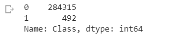
# as you can see there are 492 fraud transactions.
data['Class'].value_counts()

X = data.drop(['Class'], axis = 1)
y = data["Class"]

Splitting train-test-data

from sklearn.model_selection import train_test_split

# split into 70:30 ratio
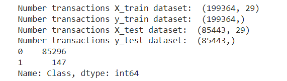
X_train, X_test, y_train, y_test = train_test_split(X, y, test_size = 0.3, random_state = 0)

# describes info about train and test set

print("Number transactions X_train dataset: ", X_train.shape)
print("Number transactions y_train dataset: ", y_train.shape)
print("Number transactions X_test dataset: ", X_test.shape)
print("Number transactions y_test dataset: ", y_test.shape)

Classification

# logistic regression object
lr = LogisticRegression()

# train the model on train set
lr.fit(X_train, y_train.ravel())
predictions = lr.predict(X_test)

# print classification report
print("Accuracy score is: ",accuracy_score(y_test, predictions))
print("Recall score is: ",recall_score(y_test, predictions))
print("Precision score is: ",precision_score(y_test, predictions))
print("Confusion Matrix: \n",confusion_matrix(y_test, predictions))

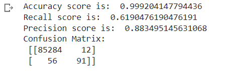
As we can see, even though the Accuracy score is 99.9%, we can see that the Recall score is 61.9% which is relatively low, and the Precision score is 88.3%.

This is because the dataset is imbalanced, and now we will try to improve these scores using the techniques mentioned above.

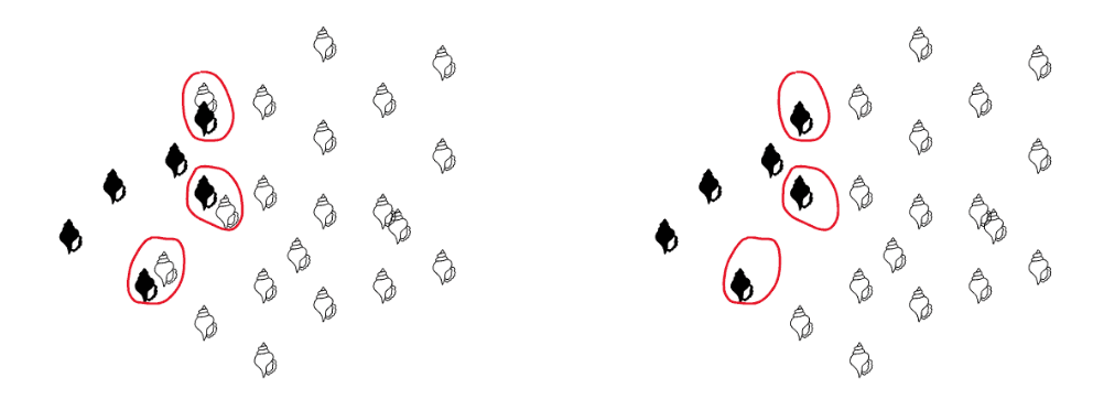
Handling Imbalanced Data using Under Sampling

Under Sampling involves the removal of records from the majority class to balance out with the minority class.

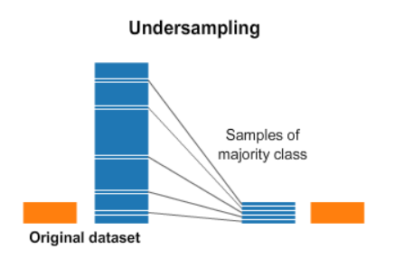
The simplest technique involved in under-sampling is Random under-sampling. This technique involves the removal of random records from the majority class. But there will be a loss of important information if we randomly remove the rows. So various techniques are implemented for undersampling the data. One such import technique is NearMiss Undersampling.

NearMiss Undersampling

In this technique, data points are selected based on the distance between the majority and minority classes. It has 3 different versions, and each version considers the different data points from the majority class.

• Version 1 — It selects data points of the majority class whose average distances to the K closest instances of minority class is the smallest
• Version 2 — It selects data points of the majority class whose average distances to the K farthest instances of minority class is the smallest
• Version 3 — It works in 2 steps. Firstly, for each minority class instance, their M nearest neighbors will be stored. Then finally, the majority class instances are selected for which the average distance to the N nearest neighbors is the largest.

In short, Version 3 is the more accurate version as it will remove the tomek links and makes the classification process easy as it forms a decision boundary.

# apply near miss
from imblearn.under_sampling import NearMiss

nr = NearMiss()

X_train_miss, y_train_miss = nr.fit_resample(X_train, y_train.ravel())

print('After Undersampling, the shape of train_X: {}'.format(X_train_miss.shape))

print('After Undersampling, the shape of train_y: {} \n'.format(y_train_miss.shape))

print("After Undersampling, counts of label '1': {}".format(sum(y_train_miss == 1)))

print("After Undersampling, counts of label '0': {}".format(sum(y_train_miss == 0)))

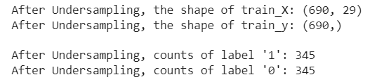
We have undersampled the majority class — 0and balanced it out with the minority class — 1. Now Let’s train and evaluate the data.

lr2 = LogisticRegression()

lr2.fit(X_train_miss, y_train_miss)

predictions = lr2.predict(X_test)

# print evaluation metrics
print("Accuracy score is: ",accuracy_score(y_test, predictions))
print("Recall score is: ",recall_score(y_test, predictions))
print("Precision score is: ",precision_score(y_test, predictions))
print("Confusion Matrix: \n",confusion_matrix(y_test, predictions))

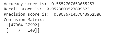
So even though the recall score is more, we can see that accuracy is less. But by our observations, when the prediction of minority class is a priority, we can use this technique.

Handling Imbalanced Data using Over Sampling

Unlike undersampling, where we remove records from the majority class, In Over sampling, we will add records in the minority class. Under-Sampling can be used when we have tons of Data, whereas Oversampling can be used when we have less Data.

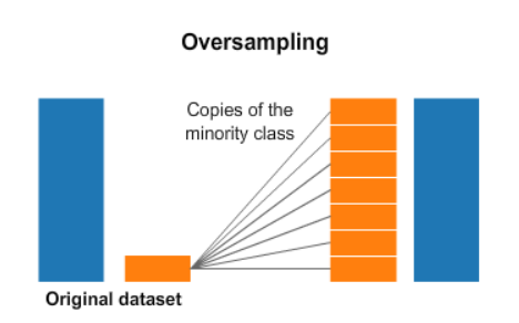
The simplest technique involved in over-sampling is Random Over Sampling, where we randomly add more copies to the minority class to balance out with the majority class, but the disadvantage of Over Sampling is that it causes overfitting and generalization of data, thereby decreasing the accuracy. So for this purpose, we use SMOTE technique.

SMOTE(Synthetic Minority Oversampling Technique)

SMOTE techniques work by randomly picking a data point from a minority class and computing the K-Nearest Neighbour from that point, and adding random points between this chosen point and its neighbors.

SMOTE Algorithm works in 4 Steps —

• Choose the minority class as the input vector.
• Find its K-Nearest Neighbours by using Euclidean distance.
• Choose one of these Neighbours and add a synthetic point between the chosen point and its Neighbours.
• Repeat the steps until it is balanced.

from imblearn.over_sampling import SMOTE

sm = SMOTE(random_state = 2)

X_train_res, y_train_res = sm.fit_resample(X_train, y_train.ravel())

print('After OverSampling, the shape of train_X: {}'.format(X_train_res.shape))
print('After OverSampling, the shape of train_y: {} \n'.format(y_train_res.shape))
print("After OverSampling, counts of label '1': {}".format(sum(y_train_res == 1)))
print("After OverSampling, counts of label '0': {}".format(sum(y_train_res == 0)))

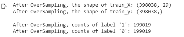
We have oversampled the minority class — 1 and balanced it out with the majority class — 0. Let’s train and evaluate the data.

lr1 = LogisticRegression()
lr1.fit(X_train_res, y_train_res.ravel())

predictions = lr1.predict(X_test)

# print Evaluation Metrics

print("Accuracy score is: ",accuracy_score(y_test, predictions))
print("Recall score is: ",recall_score(y_test, predictions))
print("Precision score is: ",precision_score(y_test, predictions))
print("Confusion Matrix: \n",confusion_matrix(y_test, predictions))

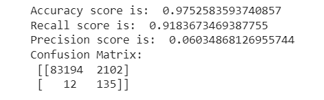
As we can see with minimal decrease in Accuracy, the recall_score has increased significantly when compared to the original statistics.

Comparing the model performance

Below is the comparison of the model without handling imbalanced data, with undersampling and with oversampling —

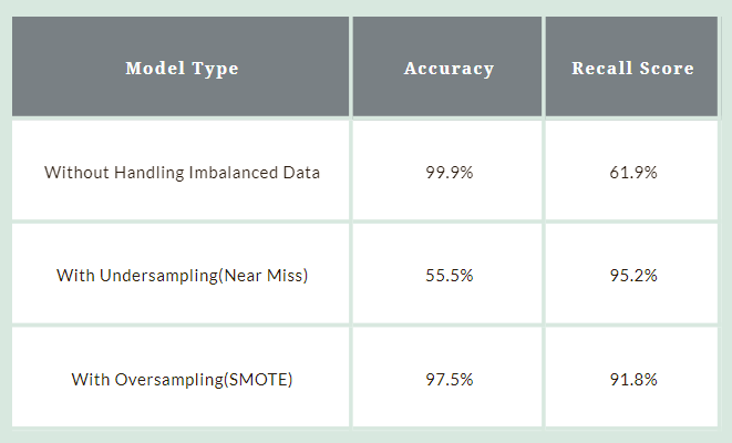
By the above metrics, one can understand that SMOTE technique has good results.

Conclusion

In this article, we have discussed how to handle Imbalanced data using different techniques. We have used Logistic regression in the above example, we can try various algorithms and improve the model performance.

I hope this is helpful…. Happy Coding…..

---

Important Techniques to Handle Imbalanced Data in Machine Learning Python was originally published in Towards AI on Medium, where people are continuing the conversation by highlighting and responding to this story.

Join thousands of data leaders on the AI newsletter. It’s free, we don’t spam, and we never share your email address. Keep up to date with the latest work in AI. From research to projects and ideas. If you are building an AI startup, an AI-related product, or a service, we invite you to consider becoming a sponsor.

Published via Towards AI