Understand the Fundamentals of an Artificial Neural Network

Author(s): Janik Tinz

Originally published on Towards AI.

Learn how an artificial neural network works

An artificial neural network (ANN) is usually implemented with frameworks such as TensorFlow, Keras or PyTorch. Such frameworks are suitable for very complex ANNs. As a data scientist, however, it is essential to understand the basics. This article aims to help you understand how a neural network works. First, we introduce the basics of an ANN in general. Then we look at the basic concepts of ANNs in detail.

Artificial Neural Networks in general

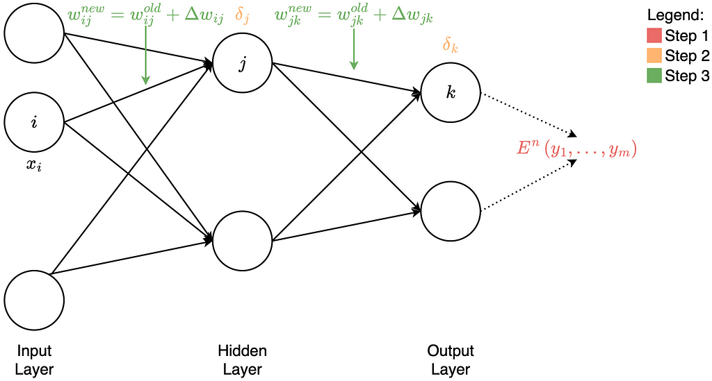
An artificial neural network uses biology as a model. Such a network consists of artificial neurons (also called nodes) and connections (also called edges) between these neurons. A neural network has one or more hidden layers, each layer consisting of several neurons. Each neuron in each layer receives the output of each neuron in the previous layer as input. Each input to the neuron is weighted. The following figure shows a Feed Forward Neural Network. In such a network, the connections between the nodes are acyclic.

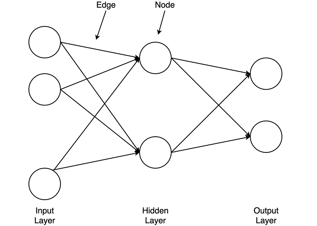
The important terms are marked in bold italics and will be looked at in more detail in this article. Feedforward is the flow of the input data through the neural network from the input layer to the output layer. As it passes through the individual layers of the network, the input data is weighted at the edges and normalized by an activation function. The weighting and the activation function are part of a neuron. The calculated values at the output of the network have an error compared to the true result values. In our training data, we know the true result values. The return of the errors is called backpropagation, where the errors are calculated per node. The gradient descent method is usually used to minimize the error terms. The training of the network with backpropagation is repeated until the network has the smallest possible error.

Then the trained neural network can use for a prediction on new data (test data). The quality of the prediction depends on many factors. As a data scientist, you need to pay attention to data quality when training a network.

Concept of a Perceptron

The concept of a perceptron was first introduced by Frank Rosenblatt in 1957. A perceptron consists of an artificial neuron with adjustable weights and a threshold. For a better understanding, we explain how a perceptron works with the following figure.

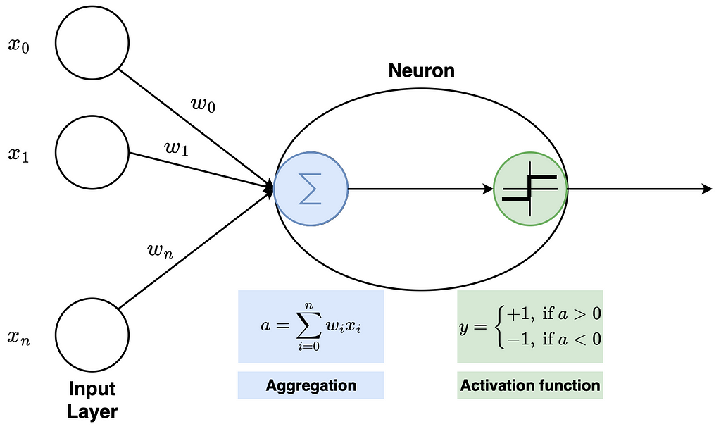
The figure illustrates an input layer and an artificial neuron. The input layer contains the input value and x_0 as bias. In a neural network, a bias is required to shift the activation function either to the positive or negative side. The perceptron has weights on the edges. The weighted sum of input values and weights is then calculated. It is also known as aggregation. The result a finally serves as input into the activation function. In this simple example, the step function is used as the activation function. Here, all values of a > 0 map to 1 and values a < 0 map to -1. There are different activation functions. Without an activation function, the output signal would just be a simple linear function. A linear equation is easy to solve, but it is very limited in complexity and has much less ability to learn a complex function mapping from data. The performance of such a network is severely limited and gives poor results.

Feedforward

Feedforward is the flow of input data through the neural network from the input layer to the output layer. This procedure explains in the following figure:

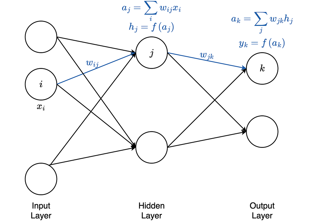
In this example, we have exactly one hidden layer. First, the data x enters into the input layer. x is a vector with individual data points. The individual data points are weighted with the weights of the edges. There are different procedures for initializing the starting weights, which we will not discuss in this article. This step is called aggregation. Mathematically, this step is as follows:

The result of this step serves as the input of the activation function. The formula is:

We denote the activation function by f. The result from the activation function finally serves as input for the neuron in the output layer.

This neuron again performs an aggregation. The formula is as follows:

The result is again the input for the activation function. The formula is:

We denote the output of the network by y. y is a vector with all y_k. The activation function in the hidden layer and the output layer does not have to be identical. In practice, different activation functions are suitable depending on the use case.

Gradient descent method

The gradient descent method minimises the error terms. In this context, the error function is derived to find a minimum. The error function calculates the error between calculated and true result values.

First, the direction in which the curve of the error function slopes most sharply must be determined. That is the negative gradient. A gradient is a multidimensional derivative of a function. Then we walk a bit in the direction of the negative slope and update the weights. The following formula illustrates this procedure:

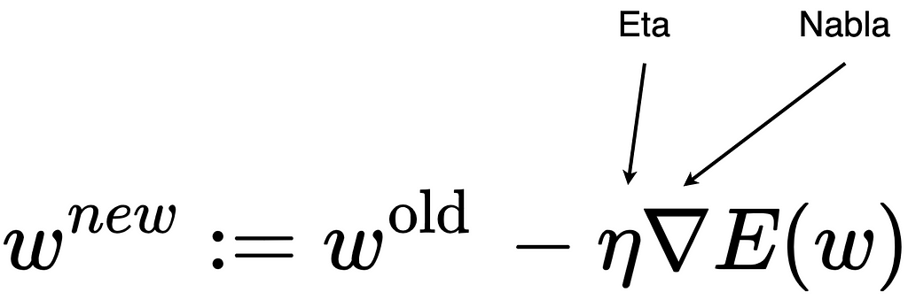
The inverted triangle is the Nabla sign and is used to indicate derivatives of vectors. The gradient descent method still requires a learning rate (Eta sign) as a transfer parameter. The learning rate specifies how strongly the weights are adjusted. E is the error function that is derived. This whole process repeats until there is no more significant improvement.

Backpropagation

In principle, backpropagation can divide into three steps.

1. Step: Construct the error function
2. Step: Calculate the error term for each node on the output and hidden layer
3. Step: Update of the weights on the edges

Construct the error function

The calculated values at the output of the network have an error compared to the true result values. An error function uses to calculate this error. Mathematically, the error can calculate in different ways. The error function contains the result from the output layer as input. That means that the whole calculation of the feedforward uses as an input to the error function. The n of the function E denotes the n-th data set. m represents the number of output neurons.

Calculate the error term for each node on the output and hidden layer

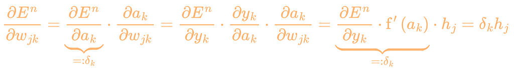
The error terms are marked orange in the Backpropagation figure. To calculate the error terms for the output layer, we have to derive the error function according to the respective weights. For this, we use the chain rule. Mathematically, it looks like this:

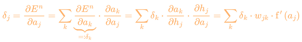
To calculate the error terms for the hidden layer, we derive the error function according to a_j.

Update of the weights on the edges

The new weights between the hidden and output layer can now calculate using the respective error terms and a learning rate. Through the minus (-), we go a bit into the direction of the descent.

The triangle is the Greek letter delta. In mathematics and computer science, this letter uses to indicate the difference. Furthermore, we can now update the weights between the input and hidden layer. The formula looks like this:

The deltas are used for the weight updates, as shown in the figure at the beginning of the Backpropagation section.

Conclusion

In this article, we have learned how an artificial neural network works. In this context, we have looked at the central concepts in detail. Feedforward describes the flow of input data through the neural network. Backpropagation is used to calculate the error terms per neuron using the gradient descent method. These concepts also build the basis for more complex network architectures.

Related literature

• Kubat, M. and Kubat, An introduction to machine learning (2019). Vol. 2. Cham, Switzerland: Springer International Publishing.
• Hastie, Trevor, et al, The elements of statistical learning: data mining, inference, and prediction (2009). Vol. 2. New York: Springer.
• Dive into Deep Learning
• A Brief Introduction to Neural Networks

Don’t miss my upcoming stories:

Get an email whenever Janik Tinz publishes.

Thanks so much for reading. If you liked this article, feel free to share it. Follow me for more content. Have a great day!

---

Understand the Fundamentals of an Artificial Neural Network was originally published in Towards AI on Medium, where people are continuing the conversation by highlighting and responding to this story.

Join thousands of data leaders on the AI newsletter. Join over 80,000 subscribers and keep up to date with the latest developments in AI. From research to projects and ideas. If you are building an AI startup, an AI-related product, or a service, we invite you to consider becoming a sponsor.

Published via Towards AI