The Normal equation: the calculus, the algebra and the code

Author(s): Menzliskander

Originally published on Towards AI.

The Normal Equation: The Calculus, the Algebra, and The Code

Introduction:

The normal equation is a closed-form solution used to solve linear regression problems. It allows us to directly compute the optimal parameters of the line (hyperplane) that best fits our data.

In this article, we’ll demonstrate the normal equation using a calculus approach and linear algebra one, then implement it in python but first, let’s recap linear regression.

Linear Regression:

let’s say we have data points x¹,x²,x³,… where each point has k features

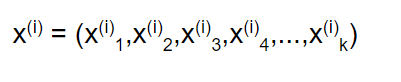
and each data point has a target value yᵢ.

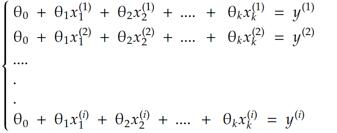
the goal of linear regression is to find parameters θ₀, θ₁, θ₂,…,θk that form a relation between each data point and it’s target value yᵢ

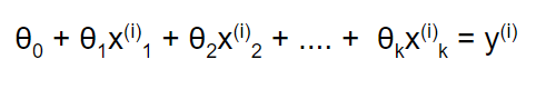
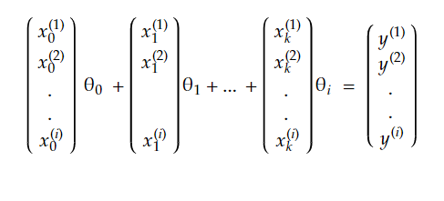
so we’re trying to solve this system of equations:

putting it all in matrix form, we get: Xθ=y with:

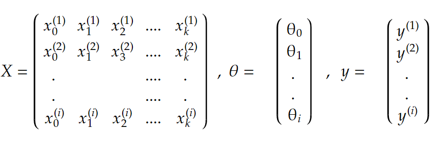
Now the problem is, in most cases, this system is not solvable. We can’t fit a straight line through the data

And this is where the normal equations will step in to find the best approximate solution, Practically the normal equation will find the parameter vector θ that solves the equation Xθ=ŷ where ŷ are as close as possible to our original target values.

and here is the normal equation:

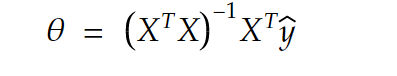
how did we get there?? Well, there are 2 ways to explain it

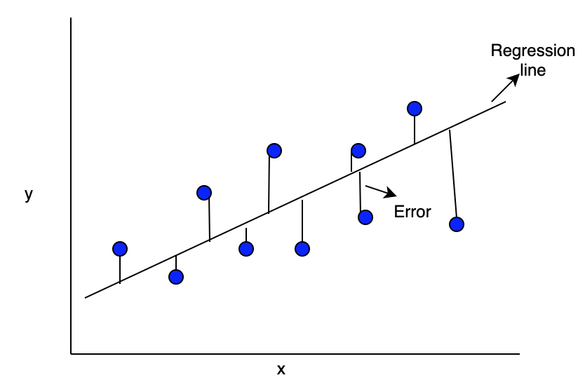
Calculus:

As we said earlier we are trying to find the parameters θ so that our predictions ŷ = Xθ is as close as possible to our original y.So we want to minimize the distance between them i.e., minimize ||y-ŷ|| and that’s the same as minimizing ||y-ŷ||² (view graph below)

now all we have to do is solve this minimization problem first, let’s expand it :

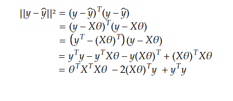
note: Xθ and y are vectors, so we can change the order when we multiply

now to find the minimum, we will derive with respect to θ and set it to 0

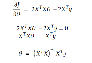
and that’s how we arrive at the normal equation. Now there is another approach that will get us there.

Linear Algebra:

Again our equation is Xθ=y, knowing a bit of matrix multiplication, we know that the result of multiplying a vector by a matrix is the linear combination of the matrix column’s multiplied by the vector’s components, so we can write as :

so for this system to have a solution, y needs to be in the column space of X (noted C(X)). And since that’s usually not the case we have to settle for the next best thing which is solving it for the closest approximation of y in C(X).

and that’s just the projection of y into C(X) !! (view image below)

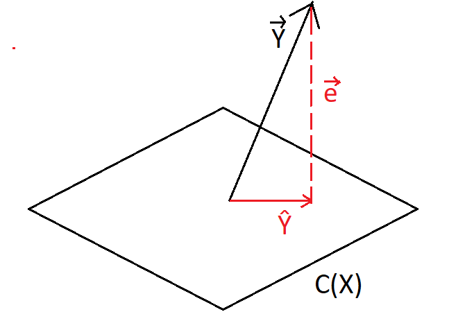
ŷ is the projection of y unto C(X) so we can write as ŷ =Xθ X^T

e = y— ŷ and since it’s orthogonal to C(X) , X^T multiplied by e is equal to 0

now putting all this to together:

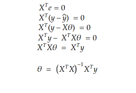
as we can see we get the same exact result!

Code:

Now implementing this in python is fairly straightforward

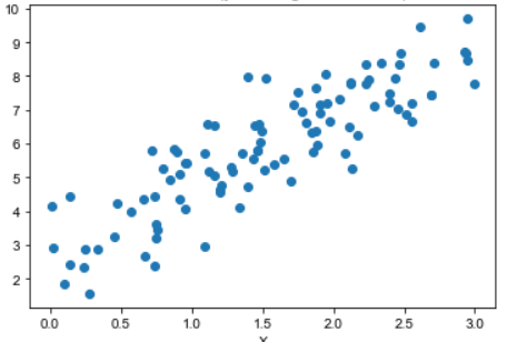
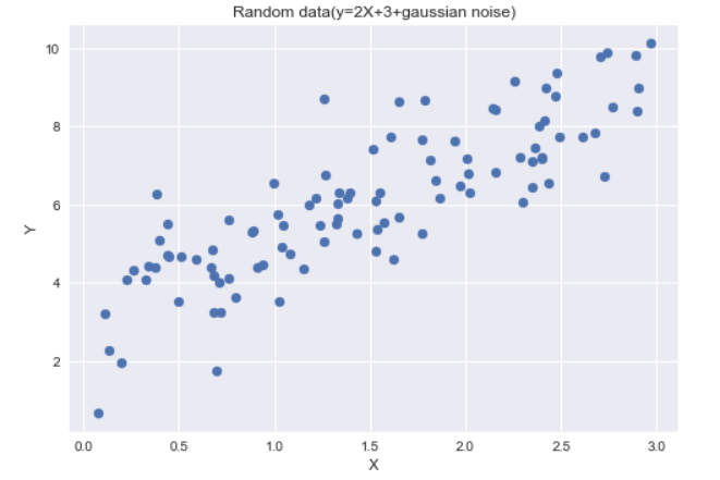
First, we’ll create some data:

import numpy as np
import matplotlib.pyplot as plt

X=3*np.random.rand(100,1)
#generating the labels using the function y=2X+3+gaussian noise
Y=2*X+3+np.random.randn(100,1)
#displaying the data
plt.scatter(X,Y)
plt.xlabel('X')
plt.ylabel('Y')
plt.title('Random data(y=2X+3+gaussian noise)')
plt.show()

#adding ones column for the bias term
X1 = np.c_[np.ones((100,1)),X]
#applying the normal equation:
theta = np.linalg.inv(X1.T.dot(X1)).dot(X1.T).dot(Y)
#we find that theta is equal to :array([[2.78609912],[2.03156946]))
#the actual function we used is y=3+2x+ gaussian noise 
#so our approximation is pretty good

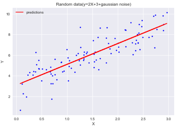
Now all that’s left is to use our θ parameters to make predictions:

Y_predict=X1.dot(theta_best)
plt.plot(X,Y,"b.")
plt.plot(X,Y_predict,"r-",label="predictions")
plt.legend()
plt.xlabel('X')
plt.ylabel('Y')
plt.title('Random data(y=2X+3+gaussian noise)')
plt.show()

Conclusion:

As we saw the normal equation is pretty straightforward and easy to use to directly get the optimal parameters however it is not commonly used on large datasets because it involves computing the inverse of the matrix which is computationally expensive (takes O(n³) time complexity) that’s why an iterative approach like gradient descent is preferred

---

The Normal equation: the calculus, the algebra and the code was originally published in Towards AI on Medium, where people are continuing the conversation by highlighting and responding to this story.

Join thousands of data leaders on the AI newsletter. Join over 80,000 subscribers and keep up to date with the latest developments in AI. From research to projects and ideas. If you are building an AI startup, an AI-related product, or a service, we invite you to consider becoming a sponsor.

Published via Towards AI