


The Parameters of Your Model Are Correlated. Now, What?
Last Updated on January 6, 2023 by Editorial Team
Last Updated on September 20, 2022 by Editorial Team
Author(s): Kevin Berlemont, PhD
Originally published on Towards AI the World’s Leading AI and Technology News and Media Company. If you are building an AI-related product or service, we invite you to consider becoming an AI sponsor. At Towards AI, we help scale AI and technology startups. Let us help you unleash your technology to the masses.
You just got yourself a nice set of data, for example, real estate prices with the characteristics of the homes. A question you could ask yourself is: How do I predict the price of a house based on its characteristics?
The first model that comes to mind would be a linear model taking the characteristics as inputs. Let’s say that we have access to the following characteristics:
- Square footage of the house
- Number of bedrooms
- Localization
- Year of construction
The problem of predicting housing prices with such datasets has been intensively studied (https://www.kaggle.com/c/house-prices-advanced-regression-techniques), and it is possible to obtain an accurate model. I am using this framework as a toy model to highlight how easily parameters can be correlated in a model. The size of the house and the number of bedrooms are correlated, but none of them can really be used to replace the other in the estimation, thus, the estimation of the model parameters could be rendered difficult. In particular, sampling methods such as Markov Chains Monte-Carlo can be inefficient when the target distribution of the parameters is unknown. If this is a problem that might not arise when estimating housing prices, it is thus necessary to have it in mind when fitting more complicated models.
In this post, I will describe the most used sampling method, Markov Chains Monte-Carlo(MCMC), and highlight potential reasons for the inefficacy of this method when parameters are correlated. In the second part, I will describe a new sampling algorithm that is unaffected by the correlation between parameters, differential evolution MCMC (DE-MCMC). In addition, I will provide some Python code samples for both of the methods.
Markov Chain Monte-Carlo
MCMC is a sampling method that has been extensively used in Bayesian statistics, especially when estimating posterior priors. In one sentence, MCMC can be considered a random walk process used to estimate a target distribution (the distribution of the parameters). The Metropolis-Hastings is the most used algorithm within the MCMC class [1].
Let’s P = (p1, p2,…) the vector of parameters of our model. Then, the algorithm picks an initial value P1 for the parameters and samples a candidate value P* using a proposal distribution P =* K(P1). One typical proposal distribution is usually a Gaussian distribution centered around P1. Afterward, the candidate P* is accepted with the probability:
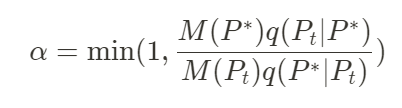
Let’s decompose this formula. M(P*) represents the target distribution. For example, in the case of a model fitting, the target distribution could be the exponential of the error function. Using the exponential function enables the switch from an error function to a probability distribution. q(Pt|P*) represents the density of the proposal distribution evaluated at Pt with parameters P*. In other words, it represents how probable it is to have selected Pt if we were to sample from P*. This term is necessary for the stationarity of the algorithm.
If the proposal is accepted, then the new starting point of the chain is P*. Otherwise, the chain does not move. This process continues until a specified number of samples has been reached. This process can be interpreted as converging to the process of sampling the target distribution and, thus, estimating the parameters P.
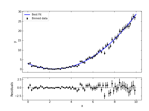
Below is a Python code sample using the package mc3 (modified from their tutorial) to simulate an MCMC algorithm to fit the parameters of a quadratic model:
Now, if we go back to the case where some of our parameters are correlated. If the proposal distribution does not explicitly take into account inter-parameter correlations, then a lot of candidate values are not going to lie within the target distribution. For example, in the figure below, the gray cloud represents a fictional distribution of two parameters. The circle represents the proposal distribution. A big part of the circle lies outside of the gray distribution.
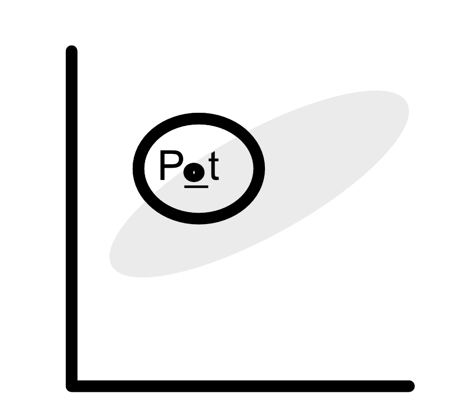
This will lead to substantial rejection rates, and the MCMC is going to be very time-consuming. Thus, it might not always be appropriate to use this Bayesian technic to fit your model. The good news is that there is a class of algorithms that can handle high-dimensional, highly correlated problems: population-based MCMC.
Diffusion Evolution Markov Chains Monte-Carlo
Differential evolution was brought to MCMC algorithms in 2006 [2]. The idea behind the method is the following. Rather than adding noise to the current candidate value in order to produce the next step, it uses multiple interacting chains to produce the candidate value. When chains have different states, they will be used to generate new proposals for other chains. Or in other words, a candidate value of one chain is based on some weighted combination of the values of the other chains.
The combination of the values is performed the following way. P_k represents the current state of the chain k. Then the candidate value, P*, is generated using the differences between the states of two chains, picked at random, P_m and P_n. In summary, the process is the following:
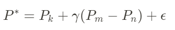
Where the factor ɣ represents the jump rate. The acceptance rate of the new candidate is similar to the MCMC algorithm, using, for example, the Metropolis-Hastings rule. A rule of thumb for using the jump rate is:
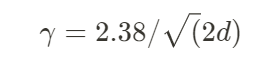
with d the number of dimensions of the parameters. The DE-MCMC algorithm is represented in the figure below:

Why is DE-MCMC efficient at sampling across correlated parameters?
The different MCMC chains are being used to inform the states in one chain. Thus, the correlations between the chains (hence correlations between samples) are being directly used to inform the states of the chains. Using the difference between chains to generate new candidate values allows for a natural way to take into account correlations between parameters. In addition, default values for the parameters of the chain work well for a variety of problems, making it a good algorithm for high-dimensional problems.
The DE-MCMC algorithm can be implemented using the MC3 package, with a sample code similar to the previous one, by specifying “demc” as the sampling algorithm of the MCMC. This leads to the following fit of the previous quadratic model:
Using the previous package to perform your MCMC algorithm, it is possible to get easy access to the posterior distributions of the parameters, pairwise correlations, and more information. If you want to look further into it, you can read their tutorial at https://mc3.readthedocs.io/en/latest/mcmc_tutorial.html#sampler-algorithm
In summary, if MCMC and Bayesian algorithms are really efficient at fitting parameters for a wide variety of models, high-dimensionality and correlation can lead to an infinite computation time. That’s when evolution algorithms come in handy. Using the differential evolution MCMC algorithm, the different chains can inform each other about parameter correlation, thus making the convergence of the algorithm faster. So, next time you have a correlation between your model parameters, try to add DE-MCMC to your set of Bayesian tools.
References
[1] Nedelman, J.R. Book review: “Bayesian Data Analysis,” Second Edition by A. Gelman, J.B. Carlin, H.S. Stern, and D.B. Rubin Chapman & Hall/CRC, 2004. Computational Statistics 20, 655–657 (2005). https://doi.org/10.1007/BF02741321
[2] Braak, Cajo J. F.. “A Markov Chain Monte Carlo version of the genetic algorithm Differential Evolution: easy Bayesian computing for real parameter spaces.” Statistics and Computing 16 (2006): 239–249.
The Parameters of Your Model Are Correlated. Now, What? was originally published in Towards AI on Medium, where people are continuing the conversation by highlighting and responding to this story.
Join thousands of data leaders on the AI newsletter. It’s free, we don’t spam, and we never share your email address. Keep up to date with the latest work in AI. From research to projects and ideas. If you are building an AI startup, an AI-related product, or a service, we invite you to consider becoming a sponsor.
Published via Towards AI
Towards AI Academy
We Build Enterprise-Grade AI. We'll Teach You to Master It Too.
15 engineers. 100,000+ students. Towards AI Academy teaches what actually survives production.
Start free — no commitment:
→ 6-Day Agentic AI Engineering Email Guide — one practical lesson per day
→ Agents Architecture Cheatsheet — 3 years of architecture decisions in 6 pages
Our courses:
→ AI Engineering Certification — 90+ lessons from project selection to deployed product. The most comprehensive practical LLM course out there.
→ Agent Engineering Course — Hands on with production agent architectures, memory, routing, and eval frameworks — built from real enterprise engagements.
→ AI for Work — Understand, evaluate, and apply AI for complex work tasks.
Note: Article content contains the views of the contributing authors and not Towards AI.
Related posts
Recent Posts


")

