The Mathematical Relationship between Model Complexity and Bias-Variance Dilemma

Author(s): Harjot Kaur

Originally published on Towards AI the World’s Leading AI and Technology News and Media Company. If you are building an AI-related product or service, we invite you to consider becoming an AI sponsor. At Towards AI, we help scale AI and technology startups. Let us help you unleash your technology to the masses.

Most data science enthusiasts will concur with the claim – the ‘Bias-variance dilemma suffers from analysis paralysis’, as there is an immense literature on the concept of Bias-Variance, its decomposition, derivation, and its relationship with model complexity. Perhaps, we have crammed to the best of our abilities that simple models exhibit high bias and complex models experience low bias. Have we ever wondered why?

Some may choose to ignore this by proclaiming it to be just another question. But, there exists an established mathematical relationship between model complexity and bias-variance dilemma. Getting a good grasp of this may help data science practitioners to conduct a proper error analysis and apply regularization techniques precisely. So, let’s dive in to understand the concept first briefly and later derive the mathematical relationship!

The Bias-Variance-Noise Decomposition

Simply put, Bias is the simplifying assumptions made by a model to make the target function easier to learn. Low bias suggests fewer assumptions about the form of the target function. High bias suggests more assumptions about the form of the target function.

Variance is the amount that the estimate of the target function will change if different training data is used. Low Variance suggests small changes to the estimate of the target function with changes to the training dataset. High Variance suggests large changes to the estimate of the target function with changes to the training dataset.

But let’s attempt to understand how this works mathematically.

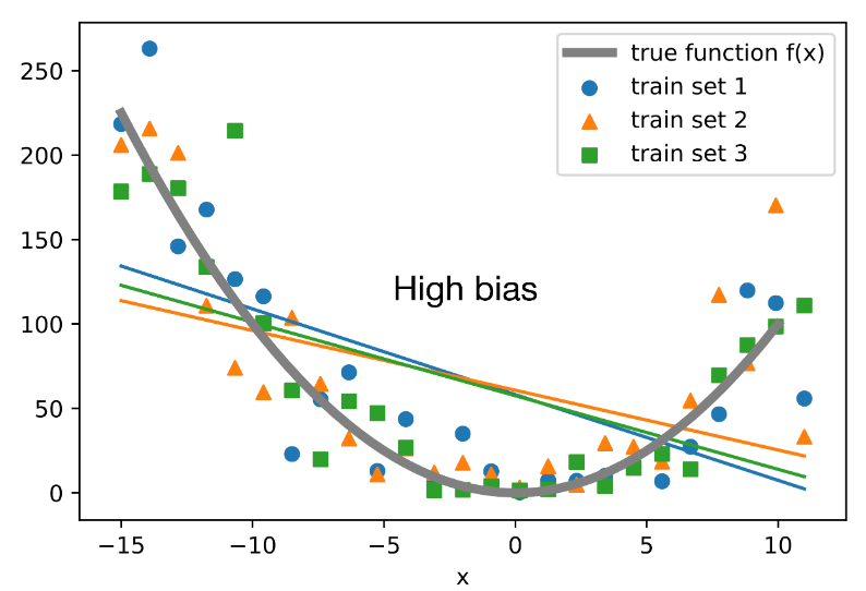
Mathematically, bias can be expressed as:

where f(x) is the true model, f^(x) is the estimate of our model, and E[f^(x)] is the average (or expected) value of the model.

This simply means bias is the difference between the expected value of the estimator and the parameter. In the graph below, a simple model(linear function) is plotted over 3 training sets, and the grey line defines the true function. We can clearly observe high bias as the average simple models are totally off the true function.

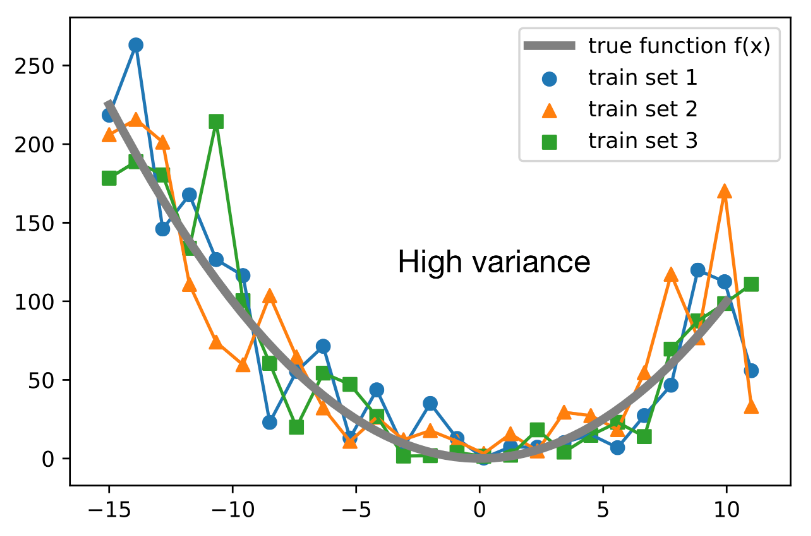
And, Variance can be given as:

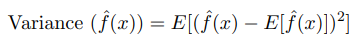
It is defined as the difference between the expected value of the squared estimator minus the squared expectation of the estimator. Again, the graph below depicts that all the training sets fit very closely to the true function, and when provided unseen data will not be able to apply its learnings. Hence, high variance!

Why is the Bias-Variance tradeoff required in the first place?

Empirical studies impress that the expected value of error is composed of bias, variance, and noise. The decomposition of the loss into bias and variance helps us understand learning algorithms, as these concepts are correlated to underfitting and overfitting. Therefore, with an inherent need to reduce the true error, we must work on optimizing its components i.e., bias and variance. Let’s take a look at the decomposition of bias-variance-noise.

Here,

• the true or target function as y=f(x),
• the predicted target value as y^=f^(x)=h(x),
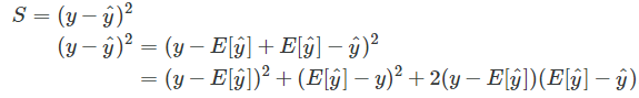
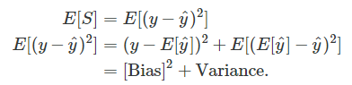
• and the squared loss as S=(y−y^)²

To get started with the squared error loss decomposition into bias and variance, let us do some algebraic manipulation, i.e., adding and subtracting the expected value of y^ and then expanding the expression using the quadratic formula (a+b)²=a²+b²+2ab):

Next, we just use the expectation on both sides, and we are already done:

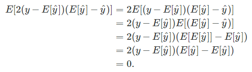
You may wonder what happened to the “2ab” term (2(y−E[y^])(E[y^]−y^) when we used the expectation. It turns that it evaluates to zero and hence vanishes from the equation, which can be shown as follows:

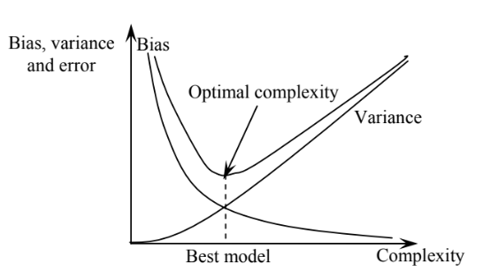
Thus, to reduce the expected error, we must select the sweet spot between high bias and high variance. That gives us the best model. As depicted in Figure3, the best model is with the optimal complexity striking a balance between bias and variance.

Now the gold question! How does model complexity impact the true error?

Let’s attempt to comprehend this using Stein’s Lemma.

where LHS represents the true error, and RHS explains a small change in the observation(yi) causes a large change in the estimation( ˆf).

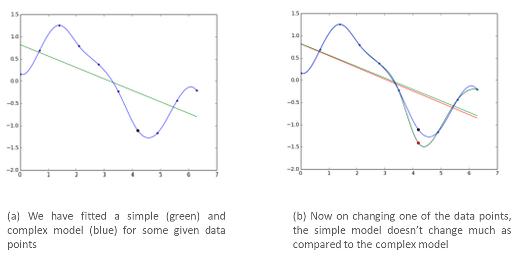
This indicates when the term on the RHS is high, a small change in an observation will cause a large change in the estimation, thereby increasing the loss. Indeed a complex model will be more sensitive to changes in observations, whereas a simple model will be less sensitive to changes in observations.

Let us verify the above claim. We have fitted a simple and complex model for some given data. Now, on changing one of the data points, the simple model doesn't change much as compared to the complex model(refer to the graphs below).

Hence, we can say that:

true error = empirical train error + small constant + Ω(model complexity)

Hence while training, instead of minimizing the training error Ltrain(θ) we should minimize

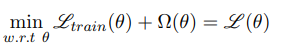
Where Ω(θ) would be high for complex models and small for simple models, and this becomes the basis for all regularization methods.

In this piece, we have covered the universally accepted definitions of bias and variance. Also, we have attempted to decompose the Bias-Variance-Noise components of the expected error mathematically. Additionally, we attempted to mathematically arrive at the equation using Stein’s lemma, which explains how model complexity impacts the expected error, i.e., bias² + variance.

I Hope this write-up was of some value to the readers, and I thank you for your patience in reading this enduring piece. Do write back with your comments or questions, and I will be happy to respond. Also, if you are keen to have interaction on data science and analytics, let’s connect on Linkedin.

References:

i) https://www.researchgate.net/publication/221434786_A_Bias-Variance-Complexity_Trade-Off_Framework_for_Complex_System_Modeling

ii) Bias-Variance tradeoff by Mitesh Khapra

iii)http://rasbt.github.io/mlxtend/user_guide/evaluate/bias_variance_decomp/

---

The Mathematical Relationship between Model Complexity and Bias-Variance Dilemma was originally published in Towards AI on Medium, where people are continuing the conversation by highlighting and responding to this story.

Join thousands of data leaders on the AI newsletter. It’s free, we don’t spam, and we never share your email address. Keep up to date with the latest work in AI. From research to projects and ideas. If you are building an AI startup, an AI-related product, or a service, we invite you to consider becoming a sponsor.

Published via Towards AI