Stable Diffusion Based Image Compression

Author(s): Matthias Bühlmann

Originally published on Towards AI the World’s Leading AI and Technology News and Media Company. If you are building an AI-related product or service, we invite you to consider becoming an AI sponsor. At Towards AI, we help scale AI and technology startups. Let us help you unleash your technology to the masses.

Stable Diffusion Based Image Compression

Stable Diffusion makes for a very powerful lossy image compression codec.

Intro

Stable Diffusion is currently inspiring the open source machine learning community as well as upsetting artists worldwide. I was curious to see what else this impactful technology release could be used for other than making professional artists and designers ponder their job security.

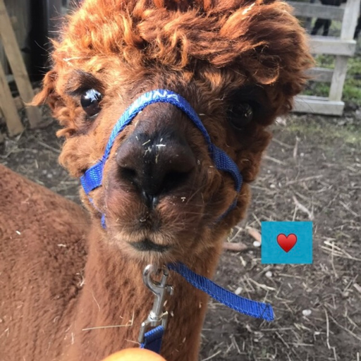
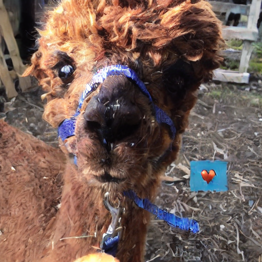
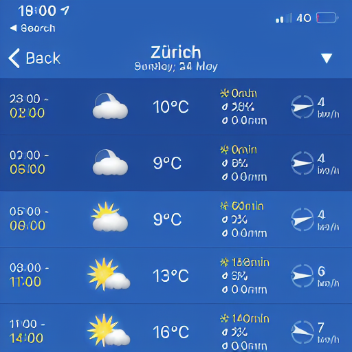
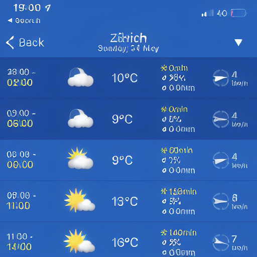
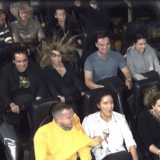
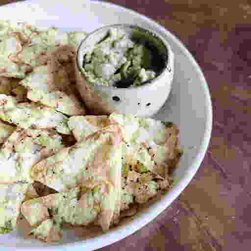
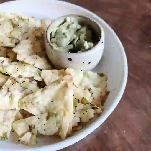
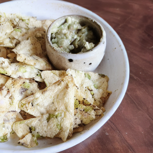
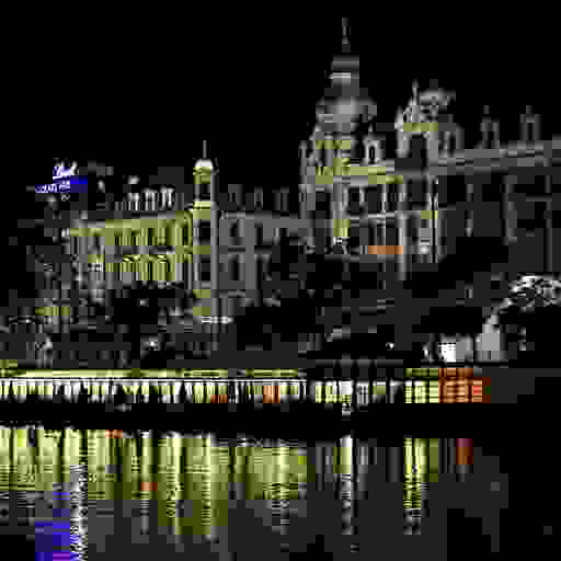
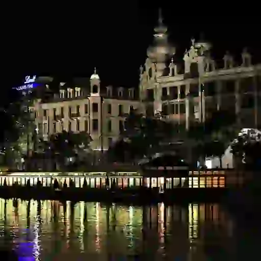
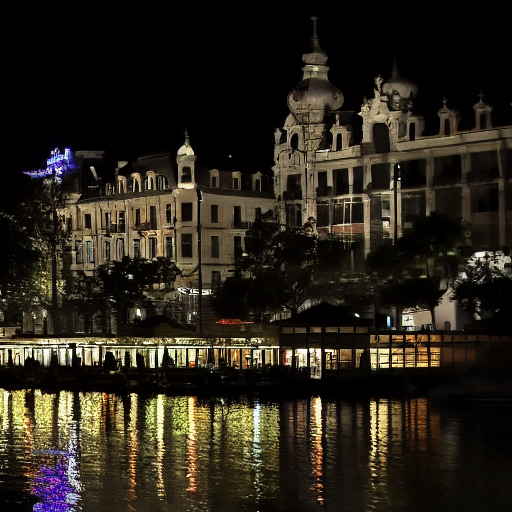
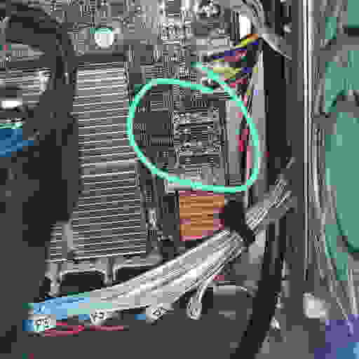
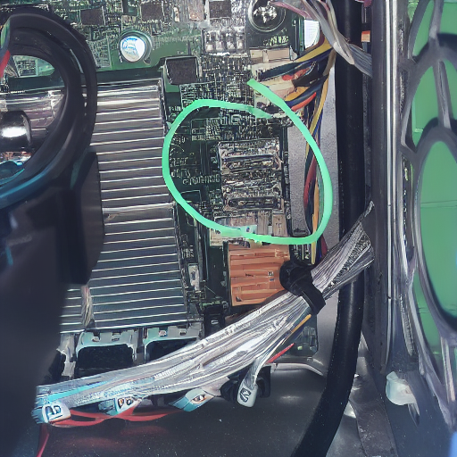
While experimenting with the model, I found that it makes for an extremely powerful lossy image compression codec. Before describing my method and sharing some code, here are a few results compared to JPG and WebP at high compression factors, all at a resolution of 512×512 pixels:

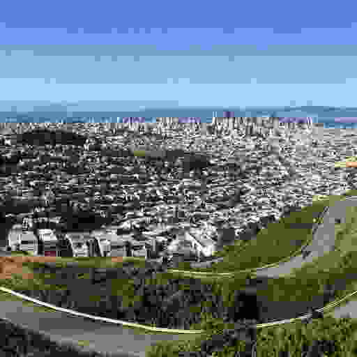
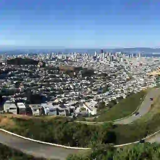
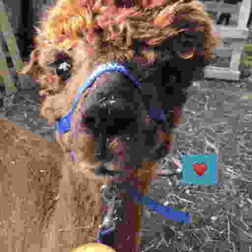
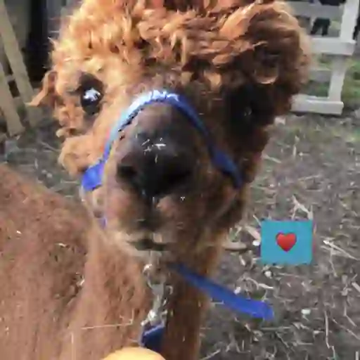
These examples make it quite evident that compressing these images with Stable Diffusion results in vastly superior image quality at smaller file size compared to JPG and WebP. This quality comes with some important caveats which must be considered, as I will explain in the evaluation section, but at a first glance, this is a very promising option for aggressive lossy image compression.

Stable Diffusion’s latent space

Stable Diffusion uses three trained artificial neural networks in tandem:

• a Variational Auto Encoder
• a U-Net
• a Text Encoder

The Variational Auto Encoder (VAE) encodes and decodes images from image space into some latent space representation. The latent space representation is a lower resolution (64 x 64), higher precision (4×32 bit) representation of any source image (512 x 512 at 3×8 or 4×8 bit).

How the VAE encodes the image into this latent space, it learns by itself during the training process and thus the latent space representations of different versions of the model will likely look different as the model gets trained further, but the representation of Stable Diffusion v1.4 looks like this (when remapped and interpreted as 4-channel color image):

The main features of the image are still visible when re-scaling and interpreting the latents as color values (with alpha channel), but the VAE also encodes the higher resolution features into these pixel values.

One encode/decode roundtrip through this VAE looks like this:

Note that this roundtrip is not lossless. For example, Anna’s name on her headcollar is slightly less readable after the decoding. The VAE of the 1.4 stable diffusion model is generally not very good at representing small text (as well as faces, something I hope version 1.5 of the trained model will improve).

The main algorithm of Stable Diffusion, which generates new images from short text descriptions, operates on this latent space representation of images. It starts with random noise in the latent space representation and then iteratively de-noises this latent space image by using the trained U-Net, which in simple terms outputs predictions of what it thinks it “sees” in that noise, similar to how we sometimes see shapes and faces when looking at clouds. When Stable Diffusion is used to generate images, this iterative de-noising step is guided by the third ML model, the text encoder, which gives the U-Net information about what it should try to see in the noise. For the experimental image codec presented here, the text encoder is not needed. The Google Colab code shared below still makes use of it, but only to create a one-time encoding of an empty string, used to tell the U-Net to do unguided de-noising during image reconstruction.

Compression Method

To use Stable Diffusion as an image compression codec, I investigated how the latent representation generated by the VAE could be efficiently compressed. Downsampling the latents or applying existing lossy image compression methods to the latents proved to massively degrade the reconstructed images in my experiments. However, I found that the VAE’s decoding seems to be very robust to quantization of the latent.

Quantizing the latents from floating point to 8-bit unsigned integers by scaling, clamping and then remapping them results in only very little visible reconstruction error:

To quantize the latents generated by the VAE, I first scaled them by 1 / 0.18215, a number you may have come across in the Stable Diffusion source code already. It seems dividing the latents by this number maps them quite well to the [-1, 1] range, though some clamping will still occur.

By quantizing the latents to 8-bit, the data size of the image representation is now 64*64*4*8 bit = 16 kB (down from the 512*512*3*8 bit= 768 kB of the uncompressed ground truth).

Quantizing the latents to less than 8-bit didn’t yield good results in my experiments, but what did work surprisingly well was to further quantize by palettizing and dithering them. I created a palettized representation using a latent palette of 256 4*8-bit vectors and Floyd-Steinberg dithering. Using a palette with 256 entries allows to represent each latent vector using a single 8-bit index, bringing the data size to 64*64*8+256*4*8 bit = 5 kB.

The palettized representation however now does result in some visible artifacts when decoding them with the VAE directly:

The dithering of the palettized latents has introduced noise, which distorts the decoded result. But since Stable Diffusion is based on de-noising of latents, we can use the U-Net to remove the noise introduced by the dithering. After just 4 iterations, the reconstruction result is visually very close to the unquantized version:

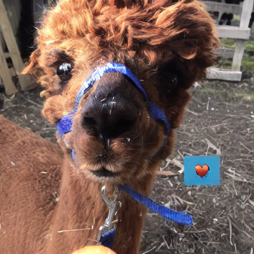
While the result is very good considering the extreme reduction in data size (a compression factor of 155x vs the uncompressed ground truth), one can also see though that artifacts got introduced, for example a glossy shade on the heart symbol that wasn’t present before compression. It’s interesting however how the artifacts introduced by this compression scheme are affecting the image content more so than the image quality, and it’s important to keep in mind that images compressed in such a way may contain these kinds of compression artifacts.

Finally, I losslessly compress the palette and indices using zlib, resulting in slightly under 5kB for most of the samples I tested on. I looked into run-length encoding, but the dithering leaves only very short runs of the same index for most images (even for those images which would work great for run-length encoding when compressed in image space, such as graphics without a lot of gradients). I’m pretty sure though there’s still even more optimization potential here to be explored in the future.

Evaluation

To evaluate this experimental compression codec, I didn’t use any of the standard test images or images found online in order to ensure that I’m not testing it on any data that might have been used in the training set of the Stable Diffusion model (because such images might get an unfair compression advantage, since part of their data might already be encoded in the trained model). Also, to make the comparison as fair as possible, I used the highest encoder quality settings for the JPG and WebP compressors of Python’s Image library and I additionally applied lossless compression of the compressed JPG data using the mozjpeg library. I then used the compression strength 1 less than what would result in a data size smaller than the Stable Diffusion result, or maximum strength otherwise (many images don’t get smaller than the SD result even at maximum lossy JPG or WebP compression).

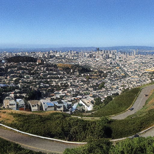
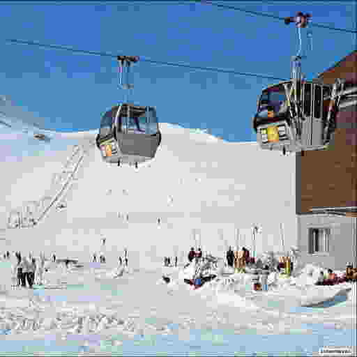
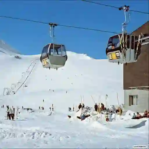
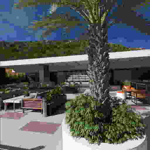
It’s important to note that while the Stable Diffusion results look subjectively a lot better than the JPG and WebP compressed images, they are not significantly better (but neither worse) in terms of standard measurement metrics like PSNR or SSIM. It’s just that the kind of artifacts introduced are a lot less notable, since they affect image content more than image quality — which however is also a bit of a danger of this method: One must not be fooled by the quality of the reconstructed features — the content may be affected by compression artifacts, even if it looks very clear. for example, looking at a detail in the San Francisco test image:

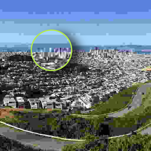
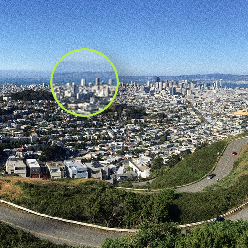
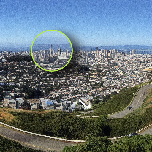
As you can see, while Stable Diffusion as codec is a lot better at preserving qualitative aspects of the image down to camera grain (something that most traditional compression algorithms struggle with), the content is still affected by compression artifacts and as such fine features such as the shape of buildings may change. While it’s certainly not possible to recognize more of the Ground Truth in the JPG compressed image than in the Stable Diffusion compressed image, the high visual quality of the SD result can be deceiving, since the compression artifacts in JPG and WebP are much more easily identified as such.

Limitations

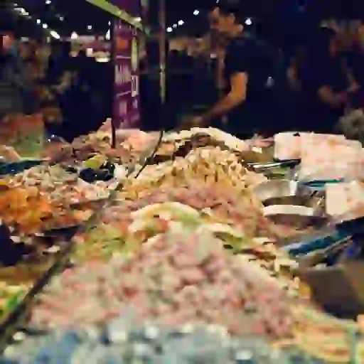
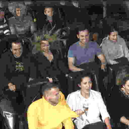
Some features are currently not well preserved by the Stable Diffusion VAE, in particular small text and faces seem to be problematic (which is consistent with the Limitations and Biases of the V1.4 SD model listed on its model card). Here are three examples that illustrate this:

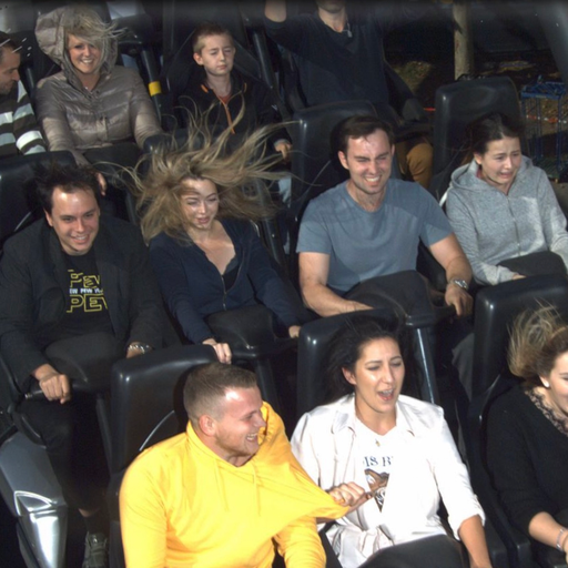
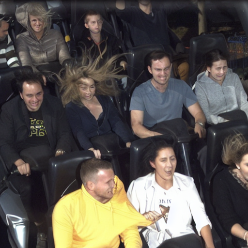
As you can see in the middle column, the current Stable Diffusion 1.4 VAE model does not preserve small text and faces very well in its latent space — as such this compression scheme inherits those limitations. But since the 1.5 version of Stable Diffusion — available so far only in stability.ai’s Dreamstudio — seems to do much better with faces, I’m looking forward to updating this article once the 1.5 model is made publicly available.

How does this approach differ from ML-based image restoration?

Deep learning is very successfully used to restore degraded images and videos or to up-scale them to higher resolution. How does this approach differ from restoring images that have been degraded by image compression?

It’s important to understand that Stable Diffusion is not used here to restore an image that has been degraded by compression in image space, but instead it applies a lossy compression to Stable Diffusion’s internal understanding of that image and then tries to ‘repair’ the damage the lossy compression caused to the internal representation (which is not the same as repairing a degraded image).

This for example preserves camera grain (qualitatively) as well as any other qualitative degradation, whereas an AI restoration of a heavily compressed jpg would not be able to restore that camera grain because any information about it has been lost from the data.

To give an analogy for this difference: Say we have a highly skilled artist who possesses a photographic memory. We show them an image and then have them recreate it and they can create an almost perfect copy just from their memory. The photographic memory of this artist is Stable Diffusion’s VAE.

In the case of restoration we would show this artist an image that has been heavily degraded by image compression and then ask them to recreate this image from memory, but in a way they think the image could have looked before it was degraded.

In the case implemented here however we show them the original, uncompressed image and ask them to memorize it as good as they can. Then we perform brain surgery on them and shrink the data in their memory by applying some lossy compression to it which removes nuances that seem unimportant and replaces very very similar variations of concepts and aspects of the memorized image by the same variation.

After the surgery we ask them to create a perfect reconstruction of the image from their memory. They’ll still remember all the important aspects of the image, from content to qualitative properties of the camera grain for example and the location and general look of every building they saw, although the exact location of every single dot of the camera grain isn’t the same anymore and some buildings they’ll remember now with weird defects that don’t really make sense.

Finally we ask them to draw the image again, but this time, if they remember some aspects in a really weird way that doesn’t make much sense to them, they should use their experience to draw these things in a way that does make sense (note that “doesn’t make sense” isn’t the same as “bad” — a blurry or scratched photo is bad, but that defect makes perfect sense).

So in both cases the artist is asked to draw things to look like what they think they should look based on their experience, but since the compression here has been applied to their memory representation of the image, which stores concepts more so than pixels, only the informational content of the concepts has been reduced, whereas in the case of restoring an image degraded by image compression both the visual quality AND the conceptual content of the image have been reduced and must be invented by the artist.

This analogy also makes it clear that this compression scheme is limited by how good the artist’s photographic memory works. In the case of Stable Diffusion v1.4 they are not very good at remembering faces and also suffer from dyslexia.

Code

If you would like to try this experimental codec yourself, you can do so with the following Google Colab:

https://colab.research.google.com/drive/1Ci1VYHuFJK5eOX9TB0Mq4NsqkeDrMaaH?usp=sharing

Conclusion

Stable Diffusion seems to be very promising as the basis for a lossy image compression scheme.

My experiments here were quite shallow, and I expect that there is a lot more potential to compressing the latent space representation beyond the technique described here, but even this relatively simple quantization and dithering scheme already yields very impressive results.

While a VAE specifically designed and trained for image compression could likely perform better on this task, the huge advantage of using the Stable Diffusion VAE is that the 6–7 figures that were already invested into Stable Diffusion’s training can be directly leveraged without having to invest vast amounts of money into training a new model for the task.

Appendix: Additional Results

---

Stable Diffusion based Image Compresssion was originally published in Towards AI on Medium, where people are continuing the conversation by highlighting and responding to this story.

Join thousands of data leaders on the AI newsletter. It’s free, we don’t spam, and we never share your email address. Keep up to date with the latest work in AI. From research to projects and ideas. If you are building an AI startup, an AI-related product, or a service, we invite you to consider becoming a sponsor.

Published via Towards AI