Gated Recurrent Neural Network from Scratch in Julia

Author(s): Jose D. Hernandez-Betancur

Originally published on Towards AI.

Let’s explore Julia to build an RNN with GRU cells from zero

1. Introduction

Julia is becoming more popular as a programming language in data science and machine learning. Julia’s popularity stems from its ability to combine the statistical strength of R, the expressive and straightforward syntax of Python, and the excellent performance of compiled languages like C++.

The best way to learn something is constant practice. This “simple” recipe is evidently effective in the tech field. Only through coding and practice can a programmer or coder grasp and explore the syntax, data types, functions, methods, variables, memory management, control flow, error handling, libraries, and best practices and conventions.

Strongly tied to this belief, I started a personal project to build a Recurrent Neural Network (RNN) that uses the state-of-the-art Gated Recurrent Units (GRUs) architecture. To add a little more flavor and increase my understanding of Julia, I built this RNN from scratch. The idea was to use the RNN with GRUs for time series forecasting related to the stock market.

Density-Based Clustering Algorithm from Scratch in Julia

Let’s code in Julia as a Python alternative in data science

pub.towardsai.net

The outline of this post is:

1. Understanding the GRU architecture
2. Setting up the project
3. Implementing the GRU network
4. Results and insights
5. Conclusion

Start, fork, share, and most crucially, experiment with the GitHub repository created for this project U+1F447.

GitHub – jodhernandezbe/post-gru-julia: This is a repository containing Julia codes to create from…

This is a repository containing Julia codes to create from scratch a Gated Recurrent Neural Network for stock…

github.com

2. Understanding the GRU architecture

The idea of this section is not to give an extensive description of the GRU architecture but to present the elements that are required to code a RNN with GRU cells from scratch. To the newcomers, I can say that RNNs belong to a family of models that enable handling sequential data like text, stock prices, and sensor data.

Unveiling the Hidden Markov Model: Concepts, Mathematics, and Real-Life Applications

Let’s explore Hidden Markov Chain

medium.com

The idea behind the GRUs is to overcome the vanishing gradient problem of the vanilla RNN. The post written by

Chi-Feng Wang can give you a simple explanation of this problem U+1F447. In case you would like to dive into the GRU, I encourage you to read the following easy-to-read and open-source papers:

1. On the Properties of Neural Machine Translation: Encoder–Decoder Approaches
2. Empirical Evaluation of Gated Recurrent Neural Networks on Sequence Modeling

The Vanishing Gradient Problem

The Problem, Its Causes, Its Significance, and Its Solutions

towardsdatascience.com

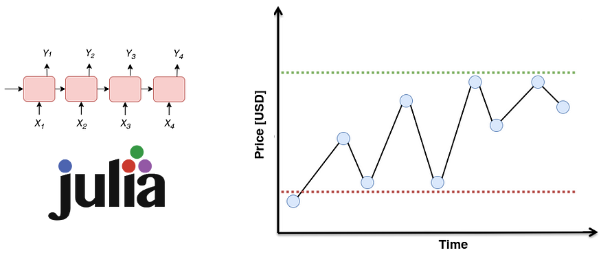
This article implements an RNN that is neither deep nor bidirectional. Julia-integrated functions must be able to capture this behavior. As illustrated in Figure 1, an RNN with GRU cells consists of a series of sequential phases. At each stage t, it supplies an element corresponding to the hidden state of the immediately preceding stage (hₜ₋₁). Similarly, an element represents the tᵗʰ element of a sample or input sequence (i.e., xₜ). The output of each GRU cell corresponds to the hidden state of that time step that will be fed to the next phase (i.e., hₜ). In addition, hₜ can be passed through a function like Softmax to obtain the desired output (for example, whether a word in a text is an adjective).

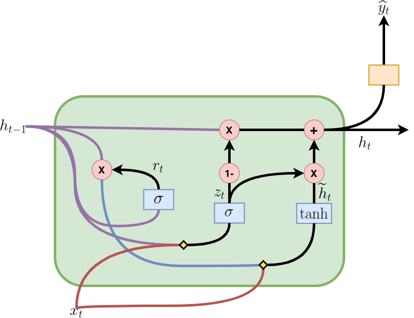
Figure 2 depicts how a GRU cell is formed, and the information flows and mathematical operations occurring inside. The cell in the time step t contains an update gate (zₜ) to determine which portion of the previous information will be passed on to the next step and a reset gate (rₜ) to determine which portion of the previous information should be forgotten. With rₜ, hₜ₋₁, and xₜ, a candidate hidden state (ĥₜ) for the current step is computed. Subsequently, using zₜ, hₜ₋₁, and ĥₜ, the actual hidden state (hₜ₋₁) is computed. All these operations make up the forward pass in a GRU cell and are summarized in the equations presented in Figure 3, where Wᵣₕ, Wᵣₓ, Wₕₕ, Wₕₓ, W₂ₓ, W₂ₕ, bᵣ, bₕ, and b₂ are the learnable parameters. The “ * ” is for matrix multiplication, while “・” for element-wise multiplication.

In the literature, it is common to find the forward-pass equations as shown in Figure 4. In this figure, matrix concatenation is used to shorten the expressions presented in Figure 3. Wᵣ, Wₕ, and W₂ are the vertical concatenations between Wᵣₕ and Wᵣₓ, Wₕₕ and Wₕₓ, and W₂ₓ and W₂ₕ, respectively. The square brackets indicate that the elements contained within them are horizontally concatenated. Both representations are useful, with the one in Figure 4 being good for shortening the formulas and the one in Figure 3 being useful for understanding the backpropagation equations.

Figure 5 shows the backpropagation equations that have to be included in the Julia program for model training. In the equations, “ T ” indicates that the matrix transposes. We can get those equations by using the definition of the total derivative for a multivariable function and the chain rule. Also, you can guide yourself by using a graphical approach U+1F447:

Forward and Backpropagation in GRUs — Derived U+007C Deep Learning

An explanation of Gated Recurrent Units (GRUs) with the math behind how the loss backpropagates through time.

medium.com

GRU units

To perform the BPTT with a GRU unit, we have the eror comming from the top layer (\(\delta 1\)), the future hidden…

cran.r-project.org

3. Setting up the project

To run the project, install Julia on your computer by following the instructions in the documentation:

Platform Specific Instructions for Official Binaries

The official website for the Julia Language. Julia is a language that is fast, dynamic, easy to use, and open source…

julialang.org

Like Python, you can use Jupyter Notebooks with Julia kernels. If you desire to do so, check out the following post written by

Dr Martin McGovern, PhD FIA:

How to Best Use Julia with Jupyter

How to add Julia code to your Jupyter notebooks and also enable you to use Python and Julia simultaneously in the same…

towardsdatascience.com

3.1. Project structure

The project inside the GitHub repository has the following tree structure:

.
├── data
│ ├── AAPL.csv
│ ├── GOOG.csv
│ └── IBM.csv
├── plots
│ ├── residual_plot.png
│ └── sequence_plot.png
├── Project.toml
├── .pre-commit-config.yaml
├── src
│ ├── data_preprocessing.jl
│ ├── main.jl
│ ├── prediction_plots.jl
│ └── scratch_gru.jl
└── tests (unit testing)
 ├── test_data_preprocessing.jl
 ├── test_main.jl
 └── test_scratch_gru.jl

Folders:

• data: In this folder, you will find .csv files containing the data to train the model. Here the files with stock prices are stored.
• plots: Folder used to store the plots that are obtained after the model training.
• src: This folder is the project core and contains the .jl files needed to preprocess the data, train the model, build the RNN architecture, create the GRU cells, and make the plots.
• tests: This folder contains the unit tests built with Julia to ensure code correctness and detect bugs. The explanation of this folder's content is beyond this article's scope. You can use it as a reference, and let me know if you would like a post exploring the Testpackage.

Unit Testing

Base.runtests(tests=["all"]; ncores=ceil(Int, Sys.CPU_THREADS / 2), exit_on_error=false, revise=false, [seed]) Run the…

docs.julialang.org

3.2. Required packages

Although we will start from scratch, the following packages are required:

• CSV(0.10.11): CSV is a package in Julia for working with Comma-Separated Values (CSV) files.
• DataFrames (1.5.0): DataFrames is a package in Julia for working with tabular data.
• LinearAlgebra (standard): LinearAlgebrais a standard package in Julia that provides a collection of linear algebra routines.
• Base (standard): Base is the standard module in Julia that provides fundamental functionality and core data types.
• Statistics (standard): Statistics is a standard module in Julia that provides statistical functions and algorithms for data analysis.
• ArgParse (1.1.4): ArgParse is a package in Julia for parsing command-line arguments. It provides an easy and flexible way to define command-line interfaces for Julia scripts and applications.
• Plots (1.38.16): Plots is a popular plotting package in Julia that provides a high-level interface for creating data visualizations.
• Random (standard):Random is a standard module in Julia that provides functions for generating random numbers and working with random processes.
• Test (standard, unit testing only): Test is a standard module in Julia that provides utilities for writing unit tests (beyond this article’s scope).

By using Project.toml, one can create an environment containing the above packages. This file is like the requirements.txt in Python or the environment.yml in Conda. Run the following command to install the dependencies:

julia --project=. -e 'using Pkg; Pkg.instantiate()'

3.3. Stock prices

As a data science practitioner, you understand that data is the fuel that powers every machine learning or statistical model. In our example, the domain-specific data is from the stock market. Yahoo Finance provides publicly available stock market statistics. We will specifically look at historical statistics for Google Inc. (GOOG). Nonetheless, you may search for and download data for other companies, such as IBM and Apple.

Alphabet Inc. (GOOG) Stock Historical Prices & Data – Yahoo Finance

Discover historical prices for GOOG stock on Yahoo Finance. View daily, weekly or monthly format back to when Alphabet…

finance.yahoo.com

4. Implementing the GRU network

Inside the folder src, you can dive into the files used to generate the plots that will be presented in Section 5 (prediction_plots.jl), process the stock prices before the model training (data_preprocessing.jl), train and build the GRU network (scratch_gru.jl), and integrate all of the above files at once (main.jl). In this section, we will delve into the four functions that compose the heart of the GRU network architecture and are the ones used to implement forward pass and backpropagation during the training.

4.1. gru_cell_forward function

The code snippet presented below corresponds to thegru_cell_forward function. This function receives the current input (x), the previous hidden state (prev_h), and a dictionary of parameters as inputs (parameters). With the above parameters, this function enables one step of GRU cell forward propagation and computes the update gate (z), the reset gate (r), the new memory cell or candidate hidden state (h_tilde), and the next hidden state (next_h), using the sigmoid and tanh functions. It also computes the prediction of the GRU cell (y_pred). Inside this function, the equations presented in Figures 3 and 4 are implemented.

4.2. gru_forward function

Unlike gru_cell_forward, gru_forward performs the forward pass of the GRU network, i.e., the forward propagation for a sequence of time steps. This function receives the input tensor (x), the initial hidden state (ho), and a dictionary as input (parameters).

If you are new to sequential models, don’t confuse a time step with the iterations so that the model error can be minimized.

Don’t confuse the x that gru_cell_forward receives with the one that gru_forward receives. In gru_forward, x has three dimenions instead of two. The third dimension corresponds to the total GRU cells that the RNN layer has. In short, gru_cell_forward is related to Figure 2, while gru_forward is related to Figure 1.

gru_forward iterates over each time step in the sequence, calling the gru_cell_forward function to compute next_h and y_pred. It stores the results in h and y, respectively.

4.3. gru_cell_backward function

gru_cell_backward performs the backward pass for a single GRU cell. gru_cell_forward receives the gradient of the hidden state (dh) as input, accompanied by the cache that contains the elements required to calculate the derivatives in Figure 5 (i.e., next_h, prev_h, z, r, h_tilde, x, and parameters). In this way, gru_cell_backward computes the gradients for the weights matrices (i.e., Wz, Wr, and Wh) and the biases (i.e., bz, br, and bh). All the gradients are stored in a Julia dictionary (gradients).

4.4. gru_backward function

gru_backward performs the backpropagation for the complete GRU network, i.e., for the complete sequence of time steps. This function receives the gradient of the hidden state tensor (dh) and the caches. Unlike in the case of gru_cell_backward, dh for gru_backward has a third dimension corresponding to the total number of time steps in the sequence or GRU cells in the GRU network layer. This function iterates over the time steps in reverse order, calling gru_cell_backward to compute the gradients for each time step, accumulating them across the loop.

It is crucial to note at this stage that this project just uses gradient descent to update the GRU network parameters and does not include any functionality that affects the learning rate or introduces momentum. Furthermore, the implementation was created with a regression concern in mind. Nonetheless, due to the modularization implemented, just little changes are required to acquire a different behavior.

5. Results and insights

Now let’s run the code to train the GRU network. Due to the integration of the ArgParse package, we can use command-line arguments to run the code. The procedure is the same if you are familiar with Python. We will perform the experiment using a training split of 0.7 (split_ratio), a sequence length of 10 (seq_length), a hidden size of 70 (hidden_size), 1000 epochs (num_epochs), and a learning rate of 0.00001 (learning_rate) because the purpose of this project is not to optimize the hyperparameters (which would involve the usage of extra modules). Run the following command to start the training:

julia --project src/main.jl --data_file GOOG.csv --split_ratio 0.7 --seq_length 10 --hidden_size 70 --num_epochs 1000 --learning_rate 0.00001

Although the model is trained across 1000 epochs, there is a flow control in the train_gru function that stores the best value for the parameters.

Figure 6 depicts the cost of training iterations. As can be observed, the curve has a decreasing tendency, and the model appears to be convergent around the last iterations. Because of the curvature of the curve, it is possible that further improvement could be obtained by increasing the number of epochs for training the GRU network. The external evaluation of the test set yields a mean squared error (MSE) of roughly 6.57. Although this value may not be near zero, a final conclusion cannot be drawn due to the lack of a benchmark value for comparison.

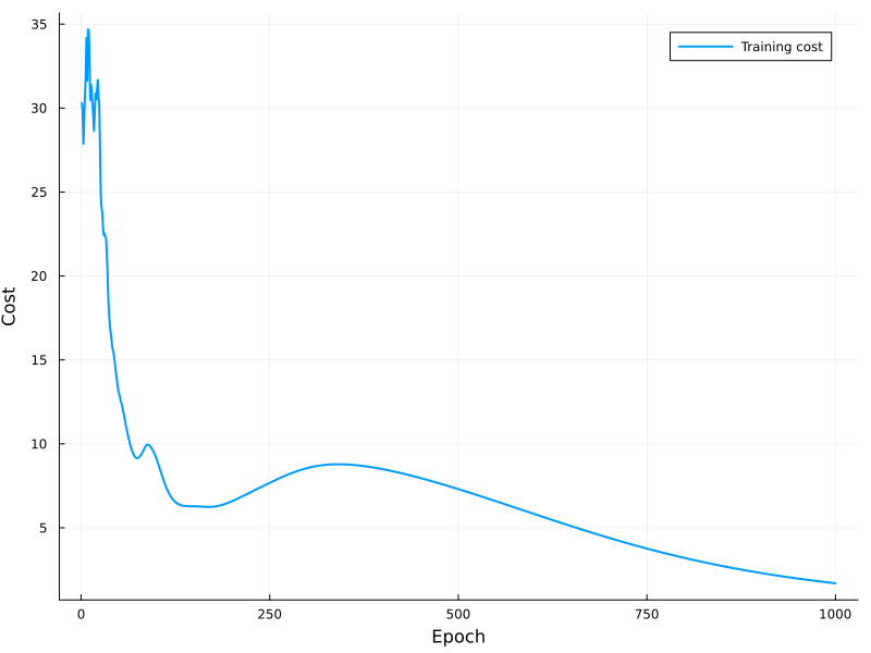
Figure 7 depicts the actual values for the training and testing datasets as scattered dots and the predicted values as continuous lines (see the figure’s legend for more details). It is clear that the model matches the actual point trend; nonetheless, more training is required to improve the GRU network’s performance. Even yet, it is feasible to see that in some portions of the picture, particularly on the training side, the model overfitted some samples; given that the MSE for the training set was around 1.70, it is possible that the model exhibits some overfitting.

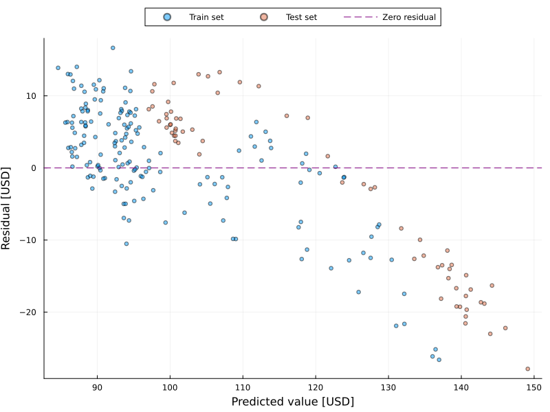
The fluctuation or instability of the error could be a difficulty in regression analysis, including time series forecasting. In data science and statistics, this is known as heteroscedasticity (for more information, check the post below U+1F447). The residual plot is one method for detecting heteroscedasticity. Figure 8 illustrates the residual plot, where the x-axis represents the predicted value and the y-axis represents the residual.

Heteroscedasticity and Homoscedasticity in Regression Learning

Variability of the residual in regression analysis

pub.towardsai.net

Dots evenly spaced around the zero value indicate the presence of homoscedasticity (i.e., stable residual). This figure shows the evidence of heteroscedasticity in this scenario, which would necessitate the use of methods to correct the problem (for example, logarithmic transformation) in order to create a high-performance model. Figure 8 shows that the presence of heteroscedasticity is evident above 120 USD, regardless of whether the sample is from the training or testing dataset. Figure 7 helps to reinforce this point. Figure 7 indicates that values greater than 120 deviate significantly from the real number.

Conclusion

In this post, we built a GRU network from zero using the Julia programming language. We began by investigating the mathematical equations that the program needed to consider, as well as the most critical theoretical issues for the GRU implementation to be successful. We went over how to create the initial settings for the Julia programs to handle the data, establish the GRU architecture, train the model, and evaluate the model. We went over the most crucial code snippets used in the design of the model architecture. We ran the programs in order to analyze the outcomes. We detected the presence of heteroscedasticity in this particular project, recommending the investigation of strategies to overcome this problem and create a high-performance GRU network.

I invite you to examine the code on GitHub and let me know if you’d like us to look at something else in Julia or another data science or programming topic. Your thoughts and feedback are extremely helpful to me U+1F680…

If you enjoy my posts, follow me on Medium to stay tuned for more thought-provoking content, clap this publication U+1F44F, and share this material with your colleagues U+1F680…

Get an email whenever Jose D. Hernandez-Betancur publishes.

Get an email whenever Jose D. Hernandez-Betancur publishes. Connect with Jose if you enjoy the content he creates! U+1F680…

medium.com

Additional material

1. Gated Recurrent Unit (GRU)
2. Sequence Models Complete Course

Join thousands of data leaders on the AI newsletter. Join over 80,000 subscribers and keep up to date with the latest developments in AI. From research to projects and ideas. If you are building an AI startup, an AI-related product, or a service, we invite you to consider becoming a sponsor.

Published via Towards AI