A Peak at How the Brain can Perform Principal Component Analysis.

Author(s): Kevin Berlemont, PhD

Originally published on Towards AI the World’s Leading AI and Technology News and Media Company. If you are building an AI-related product or service, we invite you to consider becoming an AI sponsor. At Towards AI, we help scale AI and technology startups. Let us help you unleash your technology to the masses.

The brain and the modern world have one thing in common: outputs arise from the analysis of huge information datasets. One of the most well-known data analysis methods is called Principal component analysis or PCA. The goal of this method is to transform an input into a new representation in which the variables are pairwise decorrelated. In other words, this method removes redundancy in a dataset.

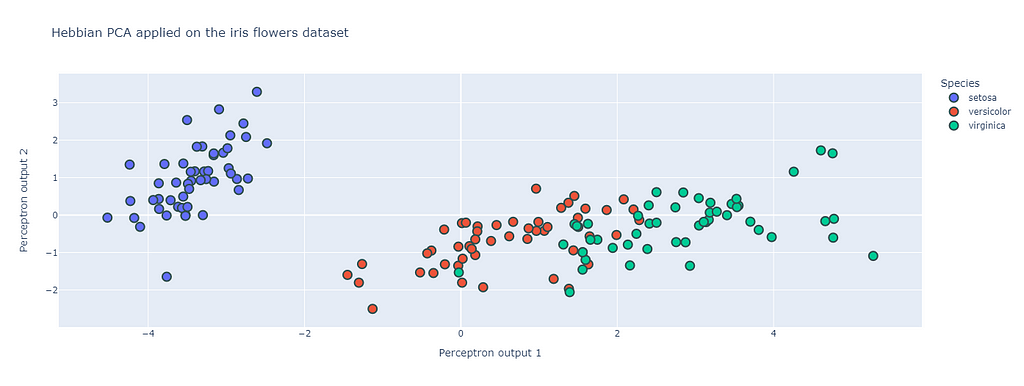
The figure above represents the PCA method applied on the open-source iris flower dataset (https://scikit-learn.org/stable/auto_examples/datasets/plot_iris_dataset.html). This dataset will be the one used in this post as an example. Despite it simplicity it will allow for a good explanation of the different methods.

One can see that in the PCA space the different species are clearly identifiable. PCA is a useful tool for analyzing structure in data, but it is subject to some limitations. I would say that one of the main one is that the PCA vectors that will form the basis of the PCA space have to be orthogonal. There is however no reason for it to be appropriate to all datasets. Still, PCA consists in one of the fundamental blocks of more advanced data analysis techniques.

In recent years, numerous works have shown that the response properties of neurons at early stages of the visual system are similar to a redundancy reduction technique for natural images. Neurons in the brain are not independent but are connected to each other. These neuronal connections are not static and their dynamics is called synaptic plasticity. While synaptic plasticity is an active research topics in Neuroscience, this neurobiological phenomenon has started to be described by Donald Hebb in 1949:

Let us assume that the persistence or repetition of a reverberatory activity (or ‘trace’) tends to induce lasting cellular changes that add to its stability … When an axon of cell A is near enough to excite a cell B and repeatedly or persistently takes part in firing it, some growth process or metabolic change takes place in one or both cells such that A’s efficiency, as one of the cells firing B, is increased.

While this rule looks very wordy it can in fact be reduce to the following: cells that wire together, fire together. Or in other words, when neurons are active together, their synaptic connections will increase.

The Hebb rule in neuroscience can be classified as an unsupervised learning rule. Indeed, it describes a basic mechanism of neural plasticity in which a repeated stimulation due to a presynaptic neuron increases the connection to the postsynaptic neuron. I am going to use a simple neuronal model, introduced by Oja in 1982, where the model is linear and the output of the neuron is actually a linear combination of what was received.

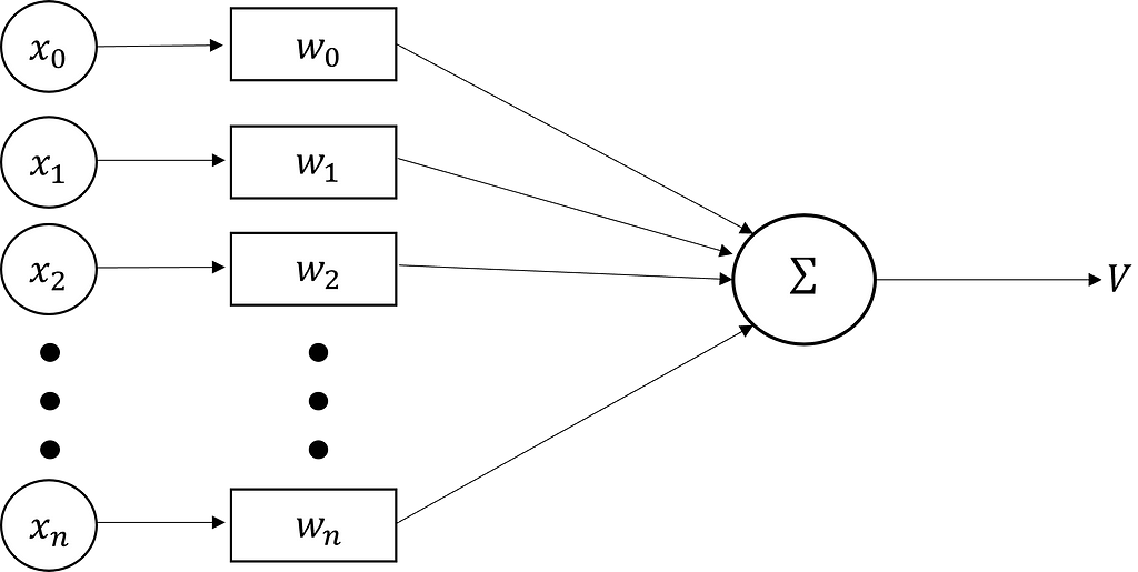
The activity V of the neuron is thus described by:

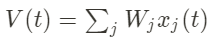
In addition, we can note that the output V(t) of the neuron is actually the scalar product of a weight vector W and an input vector x.

Now, if at every time step, the neuron receives a specific stimulus drawn from a probability distribution P, the weight vector is going to be modified according to (Hebb rule):

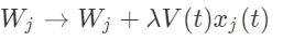
with λ a quantity called the learning rate. This learning rule corresponds to the Hebb rule as indeed if the input I and the output V are high at the same time, the weights will increase.

Geometrical interpretation

To gain some insight into what are these modifications capturing within the data distribution P, let us look at a 2-D example.

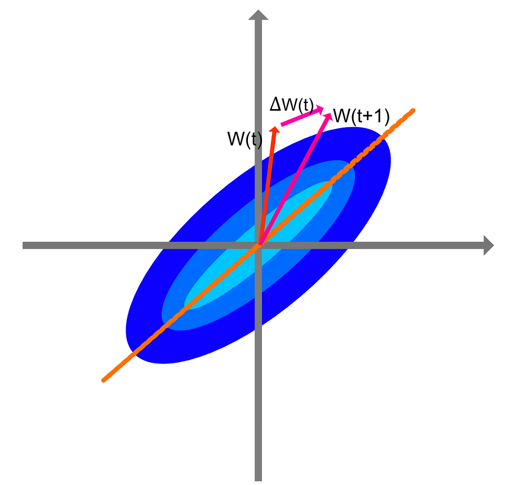
The distribution P is represented by the blue regions. Due to the strong direction of P, every iteration of the learning rule after presentation of the input is going to modify the weights W according to the red and pink arrows. The final direction of the synaptic weights vector will be the one of the maximal variance of the distribution P, or in other words, the direction in which P is the broadest. There is however an issue with this learning rule. The norm of W is not bounded as it always increases along the direction of the eigenvector of the input covariance matrix.

Constraining the growth: Oja’s rule

The idea of this rule is to modify the Hebb rule by adding a subtractive second term that will limit the growth of W.

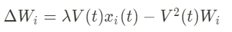
Why is this constraining rule so interesting? Once the unsupervised learning has been done, the weights follow the following equation:

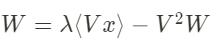
with W and x being multi-dimensional vectors. The first term of this equation can be rewritten the following way:

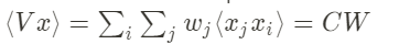
with C the input covariance matrix. Thus, we obtain:

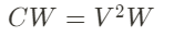
Our weight vector W is an eigenvector of C the input covariance matrix at the equilibrium. Moreover, this eigenvector is of norm 1 and it corresponds to the eigenvector with the maximum eigenvalue. The weights of this neural network move in a direction that captures the most amount of variance in the input distribution, which is the property of the first principal component.

To get more than one component, it is necessary to consider an extension Sander’s rule. First, the perceptron network will have more than one output (one per component). The next step is to implement a progressive Oja’s rule, but subtracting the predicted input for each output in a progressive manner. Thus, each weight vector learns from a different input ensemble with more structure subtracted out as they are outputs. The Python implementation of this generalized Hebbian algorithm is the following:

The function update_data computes the Hebbian learning rule, with Sander’s rule, on the weights of the network. The function is calibrated for 2 outputs (reduction at 2 dimensions).

The following figure shows that indeed the output of this 2 outputs perceptron network is indeed acting as a PCA. The structure of the projection of the dataset on the weight vectors is very similar to the first two components of the PCA, and the clusters of the three species is clearly distinguishable.

The next question one could ask on such neural networks is the following: can these networks perform more advanced methods such as clustering and independent components analysis? As the statistics that out network can learn depends on the shape of the output of the perceptron. Learning different structures requires to look at non-linear output function and thus non-linear Hebbian algorithms.

---

A Peak at How the Brain can Perform Principal Component Analysis. was originally published in Towards AI on Medium, where people are continuing the conversation by highlighting and responding to this story.

Join thousands of data leaders on the AI newsletter. It’s free, we don’t spam, and we never share your email address. Keep up to date with the latest work in AI. From research to projects and ideas. If you are building an AI startup, an AI-related product, or a service, we invite you to consider becoming a sponsor.

Published via Towards AI