A Beginner’s Guide to Markov Chains, Conditional Probability, and Independence

Author(s): Hezekiah J. Branch

Originally published on Towards AI.

Hey, everyone! I’m back with another fantastic article 😄

If you’ve followed me on LinkedIn or another platform, you may know that I’m in a graduate engineering program. Along the way, I’ve learned many fascinating topics that I hope to share with you all.

The topic I want to focus on this time is the Markov chain. Markov chains are highly popular in a number of fields, including computational biology, natural language processing, time-series forecasting, and even sports analytics. We can use Markov chains to build Hidden Markov Models (HMMs), a useful predictive model for temporal data.

If you’re new to my content, please know my tutorials are concept-focused rather than proof-heavy. I try my best to turn complicated topics into digestible nuggets.

And speaking of digestible nuggets, I introduce the Markov Chain.

A sweltering summer heat holds captive an early 1990s Boston. Inside your Egleston apartment, the sound of WCVB-TV emits from a small RCA television. You don’t believe in window AC units so you keep your window cracked with the freezer door open. Seemingly out of nowhere, a yellow envelope slides under your front door, followed by fast shuffling of feet. You wait for the sound of a closed door before picking up the envelope with caution. You’ve been hired as a private investigator to solve the disappearance of a prominent elected official. Coincidentally, you’ve already been tracking this case for some time. You walk over to your evidence board and, once again, attempt to connect the dots. For some reason, it kind of looks like a chain…

Markov chains, named after the Russian mathematician Andrey Markov, are used to model sequences of states, relying on the probability of moving from one state to the next. The term “state” can represent any number of real-world objects, including words, weather patterns, Netflix movies, you name it. This model assumes the data is ordered in some way (i.e., sequential data). Markov chain assumes that states are observable. If some of these states are not observable (i.e., hidden), we will use an HMM. It’s fairly common to refer to all of the states of the Markov chain as Q.

Quick Quiz:

If we have a Markov chain consisting of the letters of the English alphabet, how many states do we have?

Solution: The correct answer is 26! In this case, we have a state for each of the 26 letters of the alphabet.

If our states are things that we can count on our fingers (like the examples we listed above), we use the term Markov chain. If we can’t count it on our fingers (i.e., continuous), we use the term Markov process.

The key assumption behind Markov models is that we can predict the next state using only our current state. This “memoryless” assumption is called the Markov Assumption. Jurafsky and Martin (2021) give the Markov Assumption as:

The different states of our Markov chain are q1, …, qi-1 where qi-1 is our most recent state in the chain. As we learned earlier, all of these states make up Q.

The Markov Assumption above is a conditional probability distribution.

The conditional probability distribution is how we measure the probability that a variable takes on some value when we have knowledge about some other variable(s).

Like any probability distribution:

• Probability cannot be negative
• The probabilities must sum to 1
• The probability space is the sum of its disjoint parts

Real-World Example

Let’s say you’re working as a product analyst at Disney+. You may want to measure the probability that a new Marvel series will get renewed, given other variables such as average rating, number of weekly viewers, cost of production, etc. To find this probability, you’d need a conditional probability distribution.

Now if we look at the expression for the Markov Assumption, you’ll see that our conditional probability does not change when we account for additional previous states. This expression is a great example of independence versus mutual exclusivity.

When we talk about independence, we are saying that our knowledge of other variables doesn’t “update” the way we think about our variable of interest. This is different from being mutually exclusive, where two things cannot occur at the same time.

Quick Quiz:

Let A represent what you last ate for breakfast, and B represent what I last ate for breakfast. Are A and B independent, mutually exclusive, both, or neither?

Solution: If you said A and B are independent but not mutually exclusive, you’d be correct! Our breakfast choices were independent of each other because what I ate didn’t influence what I ate. However, they are not necessarily mutually exclusive because we may have eaten breakfast at the same time. These terms often get confused, but it’s important to recognize the difference between the two.

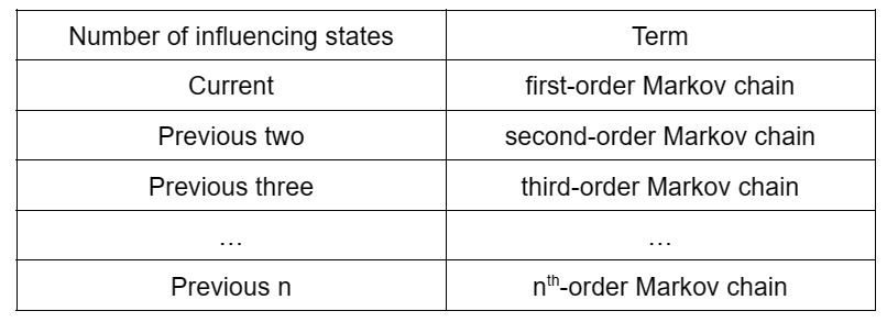
If we have a Markov chain with a conditional distribution independent of all but the most recent state, we’d call that a first-order Markov chain. If the conditional probability is independent of all but the 2 most recent states, we’d have a second-order Markov chain. If the conditional probability is independent of all but the 3 most recent states, we’d have a third-order Markov chain, and so on.

Once we have our Markov chain selected, we need to define how we move from one state to the next. Each state has a transition probability, representing the probability that we move to a given state.

We store all of these transition probabilities in the transition matrix A.

The columns and the rows of the matrix represent the states of our Markov chain. Columns of the transition matrix A form a probability distribution, so the values of each column should sum to 1. This means that all of the edges in our Markov chain leaving a state should also sum to 1. Interestingly, if each row and each column of A sum 1, we call A doubly stochastic.

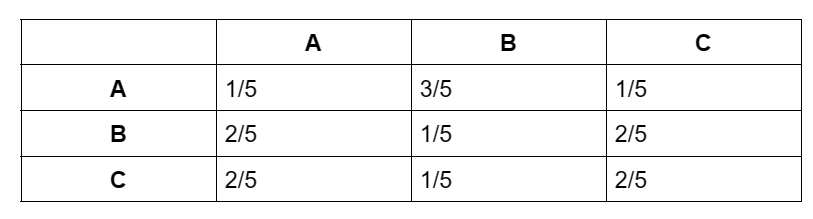
Notice how in the doubly stochastic matrix above, you can drag your finger across each row or each column and always end up with a value of 1. However, for a Markov chain, we only need the columns to add up to 1. This is called column stochastic. Such a matrix is called a left stochastic matrix. Markov chains are left stochastic but don’t have to be doubly stochastic.

Markov processes (the continuous case) can have the columns or the rows sum to 1. However, this article is strictly about Markov chains.

Quick Quiz

Below, we have an example of two proposed Markov chains. Based on what we just learned, is the left image or the right image a true Markov chain?

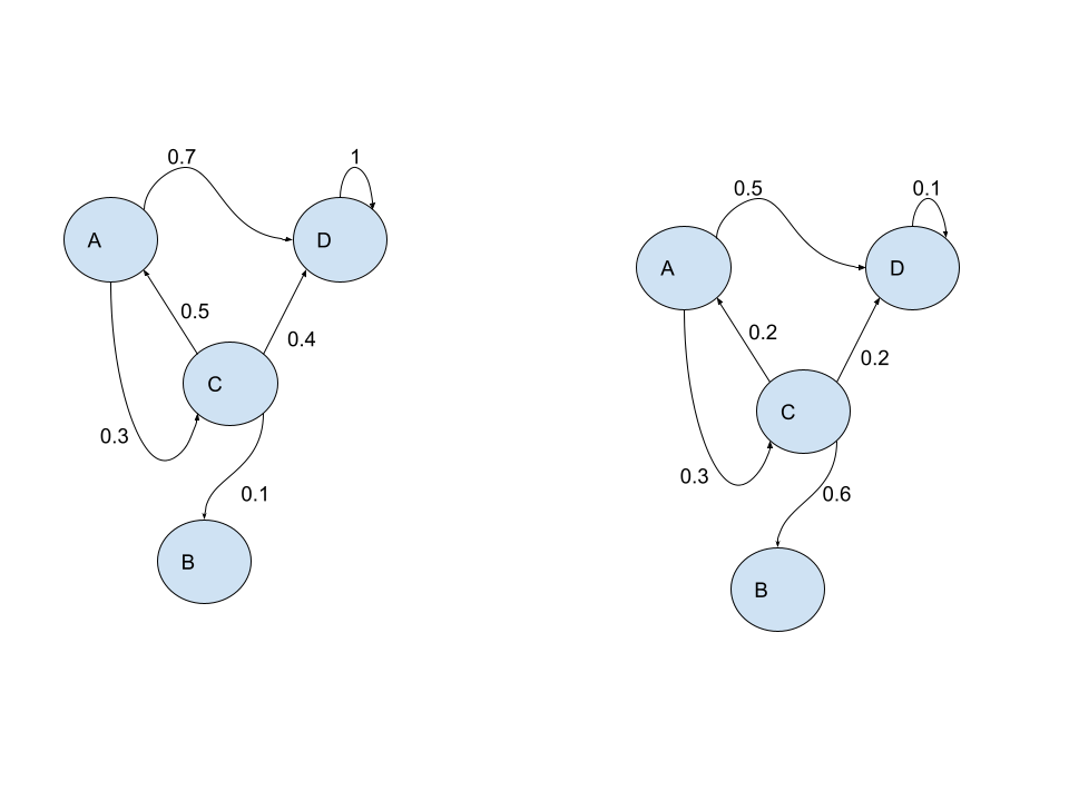
Check the end of this post for the correct answer.

Since the Markov Assumption is “memoryless,” having a meaningful representation of states is critical to the success of our model.

Activity Time: Let’s Create a Markov Chain!

Find a nearby sheet of paper and write the name of your favorite tv character. Create a Markov chain using the letters of the character’s name as states in your Markov chain. Make sure to add transition probabilities for edges between states.

Post a picture of your Markov chain and its corresponding transition matrix in the comments!

So far, we can make a Markov chain and move between states in the chain, but how do we know where to start?

This gives us our last requirement for the Markov chain, called the initial probability distribution π. This distribution is defined before any “learning” occurs. You can think of it as our “uninformed” starting point.

We multiply π by our transition matrix A to get our prediction.

An example of a prediction is given by MathAdamSpiegler below:

Here, we multiply a 3×3 transition matrix A by a 3×1 initial distribution π to get our first prediction. Notice how our prediction on the far-right sums to 1 (0.41 + 0.475 + 0.115 = 1). In this scenario, the prediction is the percentage of votes corresponding to three political candidates. The prediction above shows that Candidate 1 gets 41% of the votes, Candidate 2 gets 47.5% of the votes, and Candidate 3 gets 11.5% of the votes.

We can repeat this process a number of times to make predictions. To do so, we raise the transition matrix to some power and multiply by the initial distribution. Eventually, the prediction will hardly change. This is called a stationary distribution. Many applications of the Markov chain focus on finding the stationary distribution. However, one of the real-world limitations of the Markov chain is that it can take a while to find this stationary distribution.

Now before we depart, let’s do a brief recap of what we learned:

Summary

• Markov chains are a useful model for making predictions on sequential data, particularly when past observations are available.
• Our prediction, the conditional probability that the future state equals some value, is independent of past states of the Markov chain.
• The components of a Markov chain are the states Q, the transition matrix A, and the initial probability distribution π.
• We make predictions with our Markov chain by multiplying the transition matrix A by the initial distribution π. So, our prediction is a product equal to Aπ or ((A)^k)π where k is some power.
• Long-term predictions can be defined in terms of stationary distributions.

The solution to Markov Chain Quick Quiz:

If you look at the outgoing edges, only the left image has outgoing edges that sum to 1 for each state in the Markov chain. A has outgoing edges (0.7 + 0.3 = 1), B has no outgoing edges, C has outgoing edges (0.5 + 0.4 + 0.1 = 1), and D has one outgoing edge (1 = 1) that also acts as a loop.

If you repeat this process for the right image, you’ll find states with outgoing edges that do not sum to 1. As a result, we have an invalid probability distribution.

So, only the left image is a Markov chain!

For an interactive tutorial, check out:

(2) An Intro to Markov chains with Python! — YouTube

Next Time…

PT II: Markov Random Fields (MRFs)

— — — — — — — — — — — — — — — — — — — — — — — — — — — — — — — — — — — — — —

Sources

Speech and Language Processing. Daniel Jurafsky & James H. Martin. Copyright © 2021. All rights reserved. Draft of December 29, 2021.

Bishop, C. M., & Nasrabadi, N. M. (2006). Pattern recognition and machine learning (Vol. 4, №4, p. 738). New York: springer.

Stamp, M. (2004). A revealing introduction to hidden Markov models. Department of Computer Science San Jose State University, 26–56.

Markov chain — Wikipedia

(2) L24.2 Introduction to Markov Processes — YouTube

Math 19b: Linear Algebra with Probability Oliver Knill, Spring 2011 Lecture 33: Markov matrices

SticiGui Probability: Axioms and Fundaments (berkeley.edu)

(3) MATH 3191: Making Long Term Predictions with Markov Chains — YouTube

---

A Beginner’s Guide to Markov Chains, Conditional Probability, and Independence was originally published in Towards AI on Medium, where people are continuing the conversation by highlighting and responding to this story.

Join thousands of data leaders on the AI newsletter. Join over 80,000 subscribers and keep up to date with the latest developments in AI. From research to projects and ideas. If you are building an AI startup, an AI-related product, or a service, we invite you to consider becoming a sponsor.

Published via Towards AI