


Understanding GANs
Last Updated on August 3, 2020 by Editorial Team
Author(s): Shweta Baranwal
Deep Learning
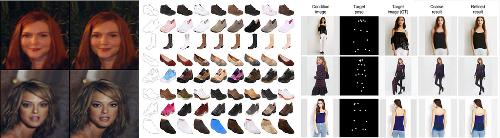
GANs (Generative Adversarial Networks) are a class of models where images are translated from one distribution to another. GANs are helpful in various use-cases, for example: enhancing image quality, photograph editing, image-to-image translation, clothing translation, etc. Nowadays, many retailers, fashion industries, media, etc. are making use of GANs to improve their business and relying on algorithms to do the task.
There are many forms of GAN available serving different purposes, but in this article, we will focus on CycleGAN. Here we will see its working and implementation in PyTorch. So buckle up!!
CycleGAN learns the mapping of an image from source X to a target domain Y. Assume you have an aerial image of a city and want to convert in google maps image or the landscape image into a segmented image, but you don’t have the paired images available, then there is GAN for you.
How is GAN different from Style Transfer? GAN is a more generalized model than Style Transfer. Here both methods try to solve the same problem, but the approach is different. Style transfer tries to keep the content of the image intact while applying the style of the other image. It extracts the content and style from the middle layers of the NN model. It focusses on learning the content and style of the image separately, but in GAN, the model tries to learn the entire mapping from one domain to another without segregating the learning of context and style.
GAN Architecture:
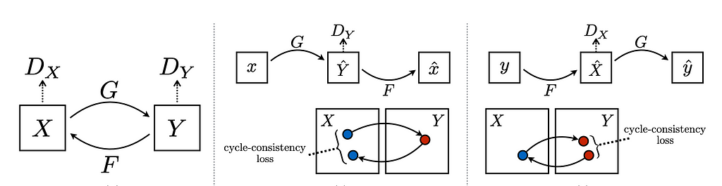
Consider two image domains, a source domain (X) and a target domain (Y). Our objective is to learn the mapping from domain G: X → Y and from F: Y → X. We have N and M training examples in domain X and Y resp.
GAN has two parts:
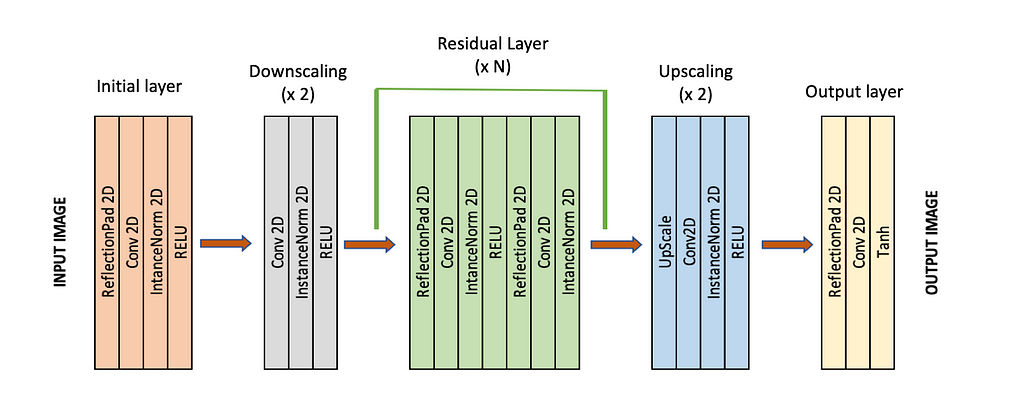
a) Generator (G)
The job of the Generator is to do the “translation” part. It learns the mapping from X → Y and Y → X and uses images in domain X to generate fake Y’s that look similar to the target domain and vice-versa. The design of Generators generally consists of downsampling layers followed by a series of residual blocks and upsampling layers.
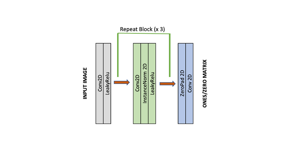
b) Discriminator (D)
The job of the Discriminator is to look at an image and output whether or not it is a real training image or a fake image from the Generator. Discriminator acts like a binary “classifier” that gives the probability of the image being real. The design of the Discriminator usually consists of a series of blocks of [conv, norm, Leaky-Relu] layers. The last layer of the Discriminator outputs the matrix, which is close to one when the input image is real else close to zero. There are two discriminators (Dx and Dy) for each domain.
During training, the Generator tries to outsmart the Discriminator by generating better and better fakes. The model reaches the equilibrium when images generated by the Generator are so good that Discriminator guesses it with almost 50% confidence, whether it’s fake or real.
Loss Function:
GAN involves three types of losses:
- Adversarial (GAN) Loss:
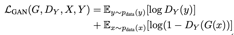
Here D(G(x)) is the probability that the output generated by G is a real image. G tries to generate the images G(x) that look similar to real image y, whereas Dy tries to distinguish between real (y) and translated (G(x)) images. D focusses on maximizing this loss function, whereas G wants to minimize this loss function, making it a minimax objective function for GAN. Similar adversarial loss follows for mapping F: Y → X.
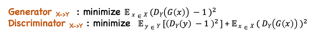
But during training, this loss function is modified into MSE loss, which is more stable and accurate. The final adversarial loss for the Generator is the sum of loss from both mappings G and F.

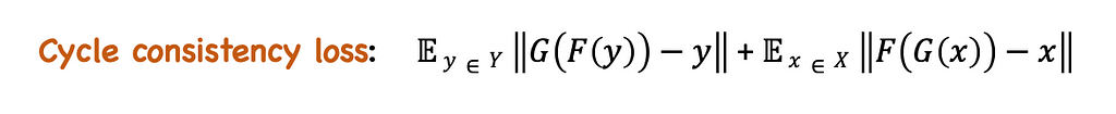
2. Cycle consistency loss:
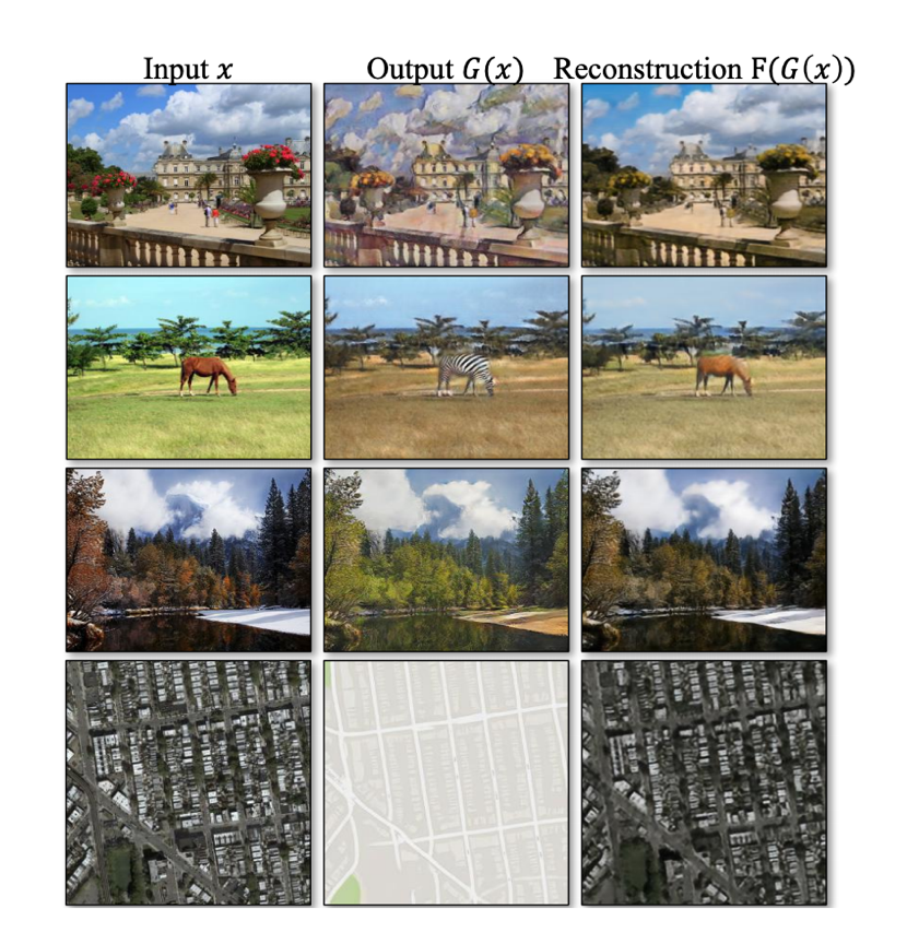
The adversarial loss function alone cannot guarantee the mapping of X to Y. It might instead learn the mapping to create an image similar to domain Y but losing all the characteristics of domain X. In order to reduce the space of possible mapping function, another loss function called cycle consistency loss is introduced. It learns to recover the original image by completing the mapping cycle of X → Y and then Y → X.
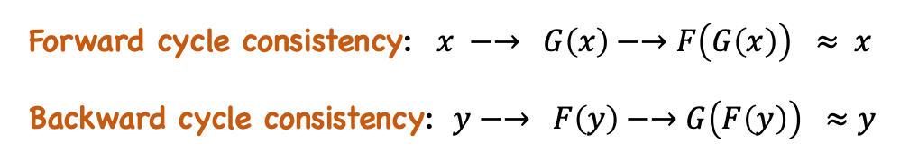
The translated image (G(x)) is passed through the mapping F to get the reconstructed image of x. The original and reconstructed images should be close enough.
3. Identity Loss:
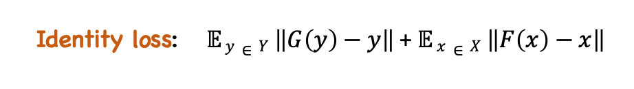
Identity loss takes care of the identity mapping of G: X → Y and F: Y → X. G(y) = y and F(x) = x
The final loss function of Generator is the weighted sum of all the above three losses.
Training
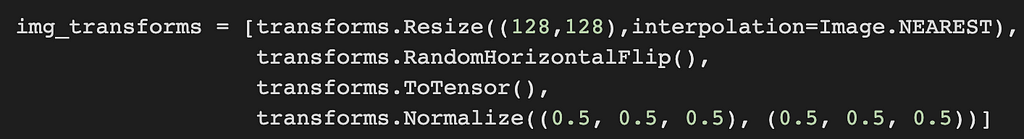
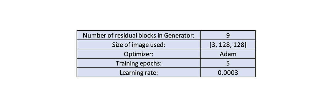
Here we are training the GAN model to do image translation from Monet’s painting to real photographs and vice-versa. The images in the dataset were of dimension 256, but due to memory constraints, the images were transformed to size 128.
Generator model used:
Discriminator model used:
Other settings:
Training steps:
Generator steps:
- Create two model instances for Generator. G_AB: Monet's to Real and G_BA: Real to Monet's. Also, two Discriminators D_A and D_B, real image classifier for both domains.
- Take a batch of images (real_A ,real_B) from domain A and B. Pass the images through G_AB and G_BA to obtain fake_B and fake_A.
- Compute the above-mentioned Generator loss and back-prop the networks G_AB and G_BA.
*Here variables valid and fake are matrices of ones and zeros, respectively.
Discriminator steps:
- Now, take the fake_A and real_A and train D_A. Use the discriminator loss function mentioned in the Adversarial loss section.
- Similarly, take fake_B and real_B and train D_B.
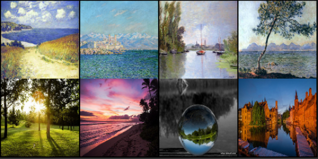
Test results:
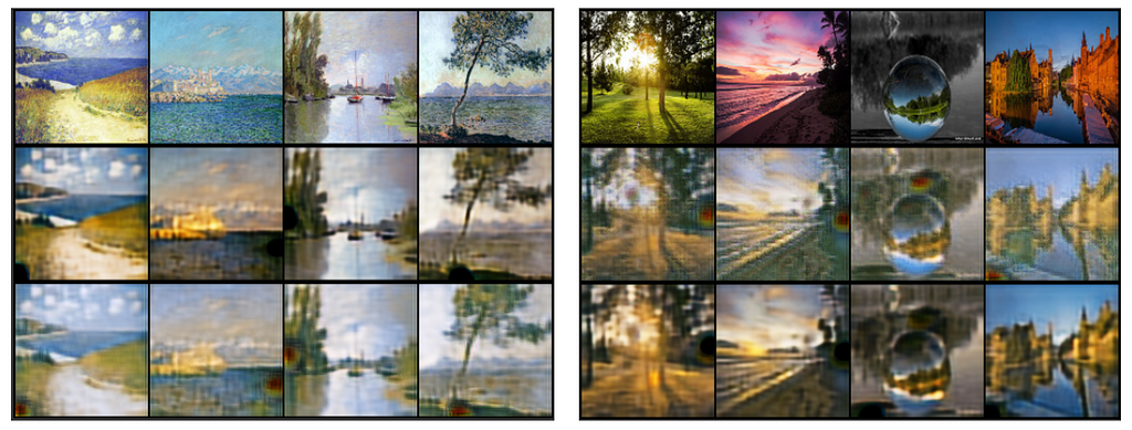
The above figures show the entire cycle of the model. Figure 1, the first row shows the real Monet’s paintings (real_A), the second row shows the conversion of Monet's painting to real photographs ( fake_B), then the third row again shows the conversion of fake_B to recover Monet's paintings (recov_A). Similarly, figure 2 shows the cycle of converting real photographs to Monet's painting and back to recovered real photos.
I am working on improving this model and learning more about GANs. Hit clap if you liked the article.
Code:
References:
- Unpaired Image-to-Image Translation using Cycle-Consistent Adversarial Networks
- Index of /~taesung_park/CycleGAN/datasets
- eriklindernoren/PyTorch-GAN
Understanding GANs was originally published in Towards AI — Multidisciplinary Science Journal on Medium, where people are continuing the conversation by highlighting and responding to this story.
Published via Towards AI
Towards AI Academy
We Build Enterprise-Grade AI. We'll Teach You to Master It Too.
15 engineers. 100,000+ students. Towards AI Academy teaches what actually survives production.
Start free — no commitment:
→ 6-Day Agentic AI Engineering Email Guide — one practical lesson per day
→ Agents Architecture Cheatsheet — 3 years of architecture decisions in 6 pages
Our courses:
→ AI Engineering Certification — 90+ lessons from project selection to deployed product. The most comprehensive practical LLM course out there.
→ Agent Engineering Course — Hands on with production agent architectures, memory, routing, and eval frameworks — built from real enterprise engagements.
→ AI for Work — Understand, evaluate, and apply AI for complex work tasks.
Note: Article content contains the views of the contributing authors and not Towards AI.
Related posts


")
Recent Posts


")

