
Principal Component Analysis (PCA) with Python Examples — Tutorial
Last Updated on November 12, 2020 by Editorial Team

An in-depth tutorial on principal component analysis (PCA) with mathematics and Python coding examples
Author(s): Saniya Parveez, Roberto Iriondo
This tutorial’s code is available on Github and its full implementation as well on Google Colab.
Table of Contents
- Introduction
- Curse of Dimensionality
- Dimensionality Reduction
- Correlation and its Measurement
- Feature Selection
- Feature Extraction
- Linear Feature Extraction
- Principal Component Analysis (PCA)
- Math behind PCA
- How does PCA work?
- Applications of PCA
- Implementation of PCA with Python
- Conclusion
Introduction
When implementing machine learning algorithms, the inclusion of more features might lead to worsening performance issues. Increasing the number of features will not always improve classification accuracy, which is also known as the curse of dimensionality. Hence, we apply dimensionality reduction to improve classification accuracy by selecting the optimal set of lower dimensionality features.
Principal component analysis (PCA) is essential for data science, machine learning, data visualization, statistics, and other quantitative fields.
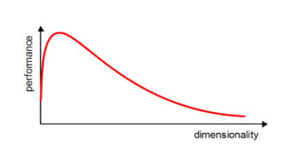
There are two techniques to make dimensionality reduction:
- Feature Selection
- Feature Extraction
It is essential to know about vector, matrix, and transpose matrix, eigenvalues, eigenvectors, and others to understand the concept of dimensionality reduction.
Curse of Dimensionality
Dimensionality in a dataset becomes a severe impediment to achieve a reasonable efficiency for most algorithms. Increasing the number of features does not always improve accuracy. When data does not have enough features, the model is likely to underfit, and when data has too many features, it is likely to overfit. Hence it is called the curse of dimensionality. The curse of dimensionality is an astonishing paradox for data scientists, based on the exploding amount of n-dimensional spaces — as the number of dimensions, n, increases.
Sparseness
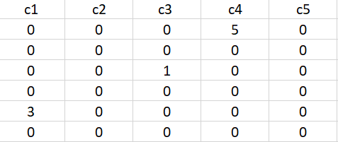
The sparseness of data is the property of being scanty or scattered. It lacks denseness, and its high percentage of the variable’s cells do not contain actual data. Fundamentally full of “empty” or “N/A” values.
Points in an n-dimensional space frequently become sparse as the number of dimensions grows. The distance between points will extend to grow as the number of dimensions increases.
Implications of the Curse of Dimensionality
There are few implications of the curse of dimensionality:
- Optimization problems will be infeasible as the number of features increases.
- Due to the absolute scale of inherent points in an n-dimensional space, as n maintains to grow, the possibility of recognizing a particular point (or even a nearby point) proceeds to fall.
Dimensionality Reduction
Dimensionality reduction eliminates some features of the dataset and creates a restricted set of features that contains all of the information needed to predict the target variables more efficiently and accurately.
Reducing the number of features normally also reduces the output variability and complexity of the learning process. The covariance matrix is an important step in the dimensionality reduction process. It is a critical process to check the correlation between different features.
Correlation and its Measurement
There is a concept of correlation in machine learning that is called multicollinearity. Multicollinearity exists when one or more independent variables highly correlate with each other. Multicollinearity makes variables highly correlated to one another, which makes the variables’ coefficients highly unstable [8].
The coefficient is a significant part of regression, and if this is unstable, then there will be a poor outcome of the regression result. Multicollinearity is confirmed by using Variance Inflation Factors (VIF). Therefore, if multicollinearity is suspected, it can be checked using the variance inflation factor (VIF).

Rules from VIF:
- A VIF of 1 would indicate complete independence from any other variable.
- A VIF between 5 and 10 indicates a very high level of collinearity [4].
- The closer we get to 1, the more ideal the scenario for predictive modeling.
- Each independent variable regresses against each independent variable, and we calculate the VIF.
Heatmap also plays a crucial role in understanding the correlation between variables.
The type of relationship between any two quantities varies over a period of time.
Correlation varies from -1 to +1
To be precise,
- Values that are close to +1 indicate a positive correlation.
- Values close to -1 indicate a negative correlation.
- Values close to 0 indicate no correlation at all.
Below is the heatmap to show how we will correlate which features are highly dependent on the target feature and consider them.
The Covariance Matrix and Heatmap
The covariance matrix is the first step in dimensionality reduction because it gives an idea of the number of features that strongly relate, and it is usually the first step in dimensionality reduction because it gives an idea of the number of strongly related features so that those features can be discarded.
It also gives the detail of all independent features. It provides an idea of the correlation between all the different pairs of features.
Identification of features in Iris dataset that are strongly correlated
Import all the required packages:
import numpy as np
import pandas as pd
from sklearn import datasets
import matplotlib.pyplot as plt
Load Iris dataset:
iris = datasets.load_iris()
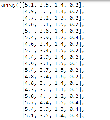
iris.data
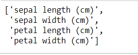
List all features:
iris.feature_names
Create a covariance matrix:
cov_data = np.corrcoef(iris.data.T)cov_data

Plot the covariance matrix to identify the correlation between features using a heatmap:
img = plt.matshow(cov_data, cmap=plt.cm.rainbow)
plt.colorbar(img, ticks = [-1, 0, 1], fraction=0.045)for x in range(cov_data.shape[0]):
    for y in range(cov_data.shape[1]):
        plt.text(x, y, "%0.2f" % cov_data[x,y], size=12, color='black', ha="center", va="center")

plt.show()
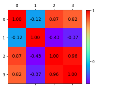
A correlation from the representation of the heatmap:
- Among the first and the third features.
- Between the first and the fourth features.
- Between the third and the fourth features.
Independent features:
- The second feature is almost independent of the others.
Here the correlation matrix and its pictorial representation have given the idea about the potential number of features reduction. Therefore, two features can be kept, and other features can be reduced apart from those two features.
There are two ways of dimensionality reduction:
- Feature Selection
- Feature Extraction
Dimensionality Reduction can ignore the components of lesser significance.
Feature Selection
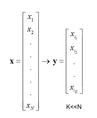
In feature selection, usually, a subset of original features is selected.
Feature Extraction
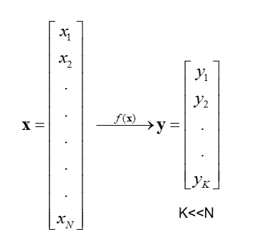
In feature extraction, a set of new features are found. That is found through some mapping from the existing features. Moreover, mapping can be either linear or non-linear.
Linear Feature Extraction
Linear feature extraction is straightforward to compute and analytically traceable.
Widespread linear feature extraction methods:
- Principal Component Analysis (PCA): It seeks a projection that preserves as much information as possible in the data.
- Linear Discriminant Analysis (LDA):- It seeks a projection that best discriminates the data.
Principal Component Analysis (PCA)
Principal Component Analysis (PCA) is an exploratory approach to reduce the data set’s dimensionality to 2D or 3D, used in exploratory data analysis for making predictive models. Principal Component Analysis is a linear transformation of data set that defines a new coordinate rule such that:
- The highest variance by any projection of the data set appears to laze on the first axis.
- The second biggest variance on the second axis, and so on.
We can use principal component analysis (PCA) for the following purposes:
- To reduce the number of dimensions in the dataset.
- To find patterns in the high-dimensional dataset
- To visualize the data of high dimensionality
- To ignore noise
- To improve classification
- To gets a compact description
- To captures as much of the original variance in the data as possible
In summary, we can define principal component analysis (PCA) as the transformation of any high number of variables into a smaller number of uncorrelated variables called principal components (PCs), developed to capture as much of the data’s variance as possible.
PCA was invented in 1901 by Karl Pearson and Harold Hotelling as an analog of the Principal axis theorem [1] [2] [3].
Mathematically the main objective of PCA is to:
- Find an orthonormal basis for the data.
- Sort dimensions in the order of importance.
- Discard the low significance dimensions.
- Focus on uncorrelated and Gaussian components.
Steps involved in PCA
- Standardize the PCA.
- Calculate the covariance matrix.
- Find the eigenvalues and eigenvectors for the covariance matrix.
- Plot the vectors on the scaled data.
Example of a problem where PCA is required
There are 100 students in a class with m different features like grade, age, height, weight, hair color, and others.
Most of the features may not be relevant that describe the student. Therefore, it is vital to find the critical features that characterize a student.
Some analysis based on the observation of different features of a student:
- Every student has a vector of data that defines him the length of m. e.g. (height, weight, hair_color, grade,….) or (181, 68, black, 99, ….).
- Each column is one student vector. So, n = 100.
- It creates an m*n matrix.
- Each student lies in an m-dimensional vector space.
Features to Ignore
- Collinear features or linearly dependent features. e.g., leg size and height.
- Noisy features that are constant. e.g., the thickness of hair
- Constant features. e.g., Number of teeth.
Features to Keep
- Non-collinear features or low covariance.
- Features that change a lot, high variance. e.g., grade.
Math Behind PCA
It is essential to understand the mathematics involved before kickstarting PCA. Eigenvalues and eigenvector play important roles in PCA.
Eigenvectors and eigenvalues
The eigenvectors and eigenvalues of a covariance matrix (or correlation) describe the source of the PCA. Eigenvectors (main components) determine the direction of the new attribute space, and eigenvalues determine its magnitude.
The PCA’s main objective is to reduce the data’s dimensionality by projecting it into a smaller subspace, where the eigenvectors form the axes. However, the eigenvectors define only the new axes’ directions because they all have a size of 1. Consequently, to decide which eigenvector(s), we can discard without losing much information in the subspace construction and checking the corresponding eigenvalues. The eigenvectors with the highest values are the ones that include more information about the distribution of our data.
Covariance Matrix
The classic PCA approach calculates the covariance matrix, where each element represents the covariance between two attributes. The covariance between two attributes is calculated as shown below:

Create a matrix:
import pandas as pd
import numpy as npmatrix = np.array([[0, 3, 4], [1, 2, 4], [3, 4, 5]])
matrix

Convert matrix to covariance matrix:
np.cov(matrix)

An exciting feature of the covariance matrix is that the sum of the matrix’s main diagonal is equal to the eigenvalues’ sum.
Correlation Matrix
Another way to calculate eigenvalues and eigenvectors is by using the correlation matrix. Although the matrices are different, they will result in the same eigenvalues and eigenvectors (shown later) since the covariance matrix’s normalization gives the correlation matrix.

Create a matrix:
matrix_a = np.array([[0.1, .32, .2,  0.4, 0.8],
             [.23, .18, .56, .61, .12],
             [.9,   .3,  .6,  .5,  .3],
             [.34, .75, .91, .19, .21]])
Convert to correlation matrix:
np.corrcoef(matrix_a.T)

How does PCA work?
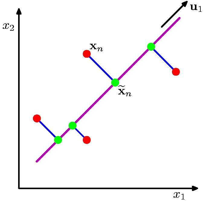
The orthogonal projection of data from high dimensions to lower dimensions such that (from figure 15):
- Maximizes the variance of the projected line (purple)
- Minimizes the MSE between the data points and projections (blue)
Applications of PCA
These are the typical applications of PCA:
- Data Visualization.
- Data Compression.
- Noise Reduction.
- Data Classification.
- Image Compression.
- Face Recognition.
Implementation of PCA with Python
Implementation of principal component analysis (PCA) on the Iris dataset with Python:
Load Iris dataset:
import pandas as pd
import numpy as np
from sklearn.datasets import load_iris
from sklearn.preprocessing import StandardScaleriris = load_iris()
df = pd.DataFrame(data=iris.data, columns=iris.feature_names)df['class'] = iris.target
df
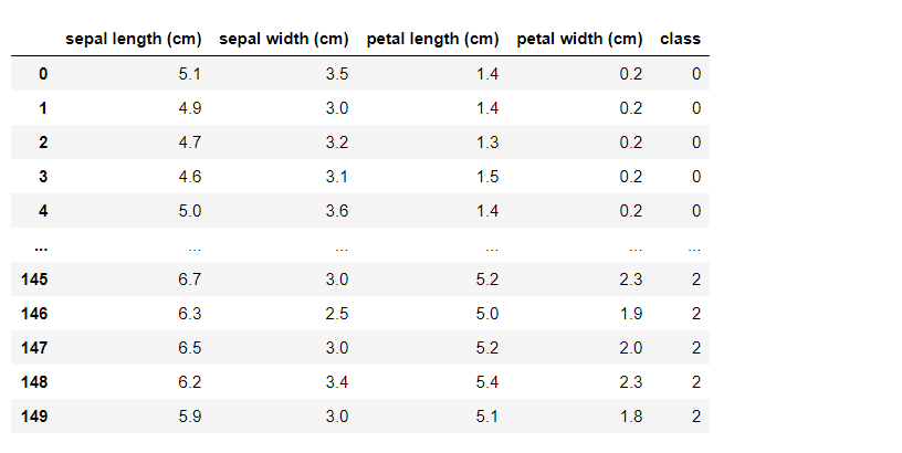
Get the value of x and y:
x = df.drop(labels='class', axis=1).values
y = df['class'].values
Implementation of PCA with a covariance Matrix:
class convers_pca():
    def __init__(self, no_of_components):
        self.no_of_components = no_of_components
        self.eigen_values = None
        self.eigen_vectors = None

    def transform(self, x):
        return np.dot(x - self.mean, self.projection_matrix.T)

    def inverse_transform(self, x):
        return np.dot(x, self.projection_matrix) + self.mean

    def fit(self, x):
        self.no_of_components = x.shape[1] if self.no_of_components is None else self.no_of_components
        self.mean = np.mean(x, axis=0)

        cov_matrix = np.cov(x - self.mean, rowvar=False)

        self.eigen_values, self.eigen_vectors = np.linalg.eig(cov_matrix)
        self.eigen_vectors = self.eigen_vectors.T

        self.sorted_components = np.argsort(self.eigen_values)[::-1]

        self.projection_matrix = self.eigen_vectors[self.sorted_components[:self.no_of_components]]self.explained_variance = self.eigen_values[self.sorted_components]
        self.explained_variance_ratio = self.explained_variance / self.eigen_values.sum()
Standardization of x:
std = StandardScaler()
transformed = StandardScaler().fit_transform(x)
PCA with two components:
pca = convers_pca(no_of_components=2)
pca.fit(transformed)
Check eigenvectors:
cov_pca.eigen_vectors
Check eigenvalues:
cov_pca.eigen_values
Check sorted component:
cov_pca.sorted_components
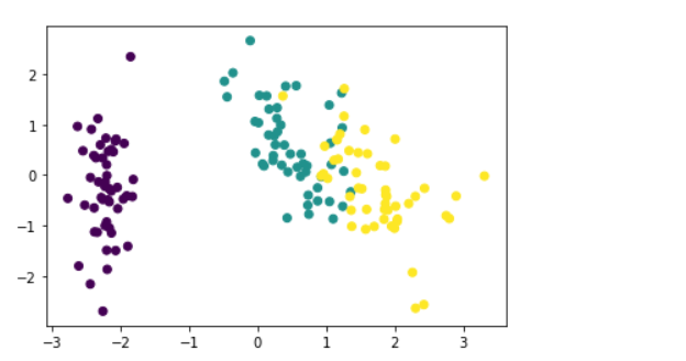
Plot PCA with several components = 2:
x_std = pca.transform(transformed)plt.figure()
plt.scatter(x_std[:, 0], x_std[:, 1], c=y)
Conclusion
Massive datasets are increasingly widespread in all sorts of disciplines. To interpret such data sets, we need to decrease dimensionality to preserve the most highly related data.
PCA solves the issue of eigenvectors/values. We apply PCA to remove colinearity during the training phase of linear regression and neural networks. PCA resembles a low-dimensional representation of the observations that explains a good fraction of the variance [6].
We can use PCA to reduce the number of variables, avoid multicollinearity, or have too many predictors relative to the number of observations. PCA is a linear combination of the p features, and taking these linear combinations of the measurements is essential to reduce the number of plots necessary for visual analysis while retaining most of the information present in the data [7].
Feature reduction is an essential preprocessing step in machine learning. Therefore, PCA is an essential step of preprocessing and very useful for compression and noise removal in the data. It reduces the dimensionality of a dataset by finding a new set of variables smaller than the original set of variables.
DISCLAIMER: The views expressed in this article are those of the author(s) and do not represent the views of Carnegie Mellon University nor other companies (directly or indirectly) associated with the author(s). These writings do not intend to be final products, yet rather a reflection of current thinking and being a catalyst for discussion and improvement.
All images are from the author(s) unless stated otherwise.
Published via Towards AI
Resources
References
[1] Pearson, K. (1901). “On Lines and Planes of Closest Fit to Systems of Points in Space”. Philosophical Magazine. 2(11): 559–572. doi:10.1080/14786440109462720.
[2] Principal Component Analysis and Optimization: A Tutorial, Robert Reris and J. Paul Brooks, https://pdfs.semanticscholar.org/e0be/f0bd8e07de281230ae5df28daabb4047e8f0.pdf
[3] Principal Component Analysis, Martin Sewell, University College London, https://citeseerx.ist.psu.edu/viewdoc/download?doi=10.1.1.325.1383&rep=rep1&type=pdf
[4] Detecting Multicollinearity Using Variance Inflation Factors, Penn State University, https://online.stat.psu.edu/stat462/node/180/
[5] Lagrange Duality and PCA CS 411 Tutorial, University of Toronto, Wenjie Luo, https://www.cs.toronto.edu/~urtasun/courses/CSC411_Fall16/tutorial7.pdf
[6] ECE 285 and SIO 209 Machine Learning for Physical Applications, Lecture 10, Peter Gerstoft, University of California San Diego, http://noiselab.ucsd.edu/ECE285/lecture10.pdf
[7] Principal Component Analysis, UC Business Analytics R Programming Guide, https://uc-r.github.io/pca
[8] Lesson 12: Multicollinearity and Other Regression Pitfalls, Regression Methods, Penn State University, https://online.stat.psu.edu/stat501/book/export/html/981
[9] Python Data Science Handbook, Jake VanderPlas, O’Reilly, https://www.oreilly.com/library/view/python-data-science/9781491912126/
Towards AI Academy
We Build Enterprise-Grade AI. We'll Teach You to Master It Too.
15 engineers. 100,000+ students. Towards AI Academy teaches what actually survives production.
Start free — no commitment:
→ 6-Day Agentic AI Engineering Email Guide — one practical lesson per day
→ Agents Architecture Cheatsheet — 3 years of architecture decisions in 6 pages
Our courses:
→ AI Engineering Certification — 90+ lessons from project selection to deployed product. The most comprehensive practical LLM course out there.
→ Agent Engineering Course — Hands on with production agent architectures, memory, routing, and eval frameworks — built from real enterprise engagements.
→ AI for Work — Understand, evaluate, and apply AI for complex work tasks.
Note: Article content contains the views of the contributing authors and not Towards AI.


