Name: Towards AI Legal Name: Towards AI, Inc. Description: Towards AI is the world's leading artificial intelligence (AI) and technology publication. Read by thought-leaders and decision-makers around the world. Phone Number: +1-650-246-9381 Email: pub@towardsai.net
228 Park Avenue South New York, NY 10003 United States
Website: Publisher: https://towardsai.net/#publisher Diversity Policy: https://towardsai.net/about Ethics Policy: https://towardsai.net/about Masthead: https://towardsai.net/about
Name: Towards AI Legal Name: Towards AI, Inc. Description: Towards AI is the world's leading artificial intelligence (AI) and technology publication. Founders: Roberto Iriondo, , Job Title: Co-founder and Advisor Works for: Towards AI, Inc. Follow Roberto: X, LinkedIn, GitHub, Google Scholar, Towards AI Profile, Medium, ML@CMU, FreeCodeCamp, Crunchbase, Bloomberg, Roberto Iriondo, Generative AI Lab, Generative AI Lab Denis Piffaretti, Job Title: Co-founder Works for: Towards AI, Inc. Louie Peters, Job Title: Co-founder Works for: Towards AI, Inc. Louis-François Bouchard, Job Title: Co-founder Works for: Towards AI, Inc. Cover:
Towards AI Cover
Logo:
Towards AI Logo
Areas Served: Worldwide Alternate Name: Towards AI, Inc. Alternate Name: Towards AI Co. Alternate Name: towards ai Alternate Name: towardsai Alternate Name: towards.ai Alternate Name: tai Alternate Name: toward ai Alternate Name: toward.ai Alternate Name: Towards AI, Inc. Alternate Name: towardsai.net Alternate Name: pub.towardsai.net
5 stars – based on 497 reviews

Frequently Used, Contextual References

TODO: Remember to copy unique IDs whenever it needs used. i.e., URL: 304b2e42315e

Resources

Take our 85+ lesson From Beginner to Advanced LLM Developer Certification: From choosing a project to deploying a working product this is the most comprehensive and practical LLM course out there!

Publication

Simple Linear Regression Tutorial for Machine Learning (ML)
Data Science   Editorial   Machine Learning   Programming   Statistics

Simple Linear Regression Tutorial for Machine Learning (ML)

Last Updated on October 21, 2021 by Editorial Team

Author(s): Pratik Shukla, Roberto Iriondo

Image for post
Source: Image by the Author.

Diving into calculating a simple linear regression and linear best fit with code examples in Python and math in detail

This tutorial’s code is available on Github and its full implementation as well on Google Colab.

Table of contents:

  1. What is a Simple Linear Regression?
  2. Calculating the Linear Best Fit
  3. Finding the equation for the Linear Best Fit
  4. Derivation of Simple Linear Regression Formula
  5. Simple Linear Regression Python Implementation from Scratch
  6. Simple Linear Regression Using Scikit-learn

What is a Simple Linear Regression?

Simple linear regression is a statistical approach that allows us to study and summarize the relationship between two continuous quantitative variables. Simple linear regression is used in machine learning models, mathematics, statistical modeling, forecasting epidemics, and other quantitative fields.

Out of the two variables, one variable is called the dependent variable, and the other variable is called the independent variable. Our goal is to predict the dependent variable’s value based on the value of the independent variable. A simple linear regression aims to find the best relationship between X (independent variable) and Y (dependent variable).

There are three types of relationships. The kind of relationship where we can predict the output variable using its function is called a deterministic relationship. In random relationships, there are no relationships between the variables. In our statistical world, it is not likely to have a deterministic relationship. In statistics, we generally have a relationship that is not so perfect, that is called a statistical relationship, which is a mixture of deterministic and random relationships [4].

Examples:

1. Deterministic Relationship:

a. Diameter = 2*pi*radius

b. Fahrenheit = 1.8*celsius+32

2. Statistical Relationship:

a. Number of chocolates vs. cost

b. Income vs. expenditure

Figure 1: A deterministic relationship vs. a statistical relationship.| Calculating linear regression and linear best fit fro
Figure 1: A deterministic relationship vs. a statistical relationship.

Understanding Simple Linear Regression:

The simplest type of regression model in machine learning is a simple linear regression. First of all, we need to know why we are going to study it. To understand it better, why don’t we start with a story of some friends that lived in “Bikini Bottom” (referencing SpongeBob) [3].

SpongeBob, Patrick, Squidward, and Gary lived in the “Bikini Bottom!”. One day Squidward went to SpongeBob, and they had this conversation. Let’s check it out.

Squidward: “Hey, SpongeBob, I have heard that you are so smart!”

SpongeBob: “Yes, sir! There is no doubt in that.”

Squidward: “Is that so?”

SpongeBob: “Umm…Yes!”

Squidward: “So here is the thing. I want to sell my house as I am going to shift to my new lavish house downtown. But I cannot figure out at which price I should sell my house! If I keep the price too high, then no one will buy it, and if I set the price low, I might face a large financial loss! So you have to help me find the best price for my house. But, please keep in mind that you have only one day!”

SpongeBob stressed as always, but optimistic about finding the solution. To discuss the problem, he went to his wise friend Patrick’s house. Patrick is in his living room watching TV with a big bowl of popcorn in his hands, and after SpongeBob described the whole situation to Patrick:

Patrick: “That is a piece of cake. Follow me!”

(They decided to go to Squidward’s neighborhood, where his two neighbors recently sold their houses. After making some discreet inquiries, they obtained the following details from Squidward’s new neighbors. Now Patrick explained the whole plan to SpongeBob.)

Patrick: Once we have some essential data on how the previous house sells from Squidward’s neighborhood, I think we can make some logical deductions to predict Squidward’s house’s price. So let us get some data.

Figure 2: Area and house price of Squidward’s neighborhood.| Calculating linear regression and linear best fit from scratch w
Figure 2: Area and house price of Squidward’s neighborhood.

From the collected data, Patrick was able to plot the data on a scatter plot:

Figure 3: Area vs. house price on a scatter plot.| Calculating linear regression and linear best fit from scratch with Python
Figure 3: Area vs. house price on a scatter plot.

If we closely observe the graph above, we can notice that we can connect our two data points with a line, and as we know, each line has its equation. From figure 3, we can quickly get the house price if we have the house’s area. It will be easier for us if we get the house price by using some formula. Please note that we can get the house price by plotting a horizontal and vertical line on the graph, but to generalize it, we use the line equation. First, we need to see some basics of geometry and dive into the equation of the line.

Basics of Coordinate Geometry:

  1. We always look from left to right in the coordinate plane to name the points.
  2. After looking from left-to-right, the first point we get must be named (x1,y1), and the second point will be (x2,y2).
  3. Horizontal lines have a slope of 0.
  4. Vertical lines have an “infinite” slope.
  5. If the second point’s Y-coordinate is greater than the Y-coordinate of the first point, then the line has a positive(+) slope. The line has a negative slope.
  6. Points at the same vertical distance from X-axis have the same Y-coordinate.
  7. Points at the same vertical distance from Y-axis have the same X-coordinate.

Now let’s get back to our graph.

We all know that the equation of the line:

Figure 4: Equation of a straight line.| Calculating linear regression and linear best fit from scratch with Python and math i
Figure 4: Equation of a straight line.

From the definition of the slope of a straight line:

Figure 5: Equation of slope of a straight line.| Calculating linear regression and linear best fit from scratch with Python
Figure 5: Equation of slope of a straight line.

From the rules mentioned above, we can infer that in our graph:

(X1 , Y1) = ( 1500 , 150000)

(X2 , Y2) = (2500 , 300000)

Next, we can easily find the slope of the two points.

Figure 6: Calculating the slope for our example.| Calculating linear regression and linear best fit from scratch with Python
Figure 6: Calculating the slope for our example.

Taking our example into consideration, in our equation, Y represents the house’s price, and X represents the area of the house.

Now since we have all the other values, we can calculate the value of slope b.

Figure 7: Calculating the Y-intercept of the line.| Calculating linear regression and linear best fit from scratch with Pytho
Figure 7: Calculating the Y-intercept of the line.

Notice that we can use any of the points to calculate the slope value. The answer to the slope will always be the same for the same straight line.
Next, since we have all our parameters, we can write the equation of line as:

Figure 8: Equation of the line.| Calculating linear regression and linear best fit from scratch with Python and math in detai
Figure 8: Equation of the line.

To find the price of Squidward’s house, we need to plug-in X=1800 in the above equation.

Figure 9: Predicting Squidward’s house price.| Calculating linear regression and linear best fit from scratch with Python and
Figure 9: Predicting Squidward’s house price.

Now, we can say that Squidward should sell his house for $ 195,000.00. That was easy.

Please note that we only had two data points to quickly plot a single straight line through them and get our equation of a line. In this case, the critical thing to notice here is that our prediction will depend on the value of two data points. If we change the value of any of the two available data points, our prediction will likely also change. To cope with this problem, we have data sets in larger quantities. Real-world datasets may contain millions of data points.

Now let us get back to our example. When we have more than two data points in our dataset(the usual case), we cannot draw a single straight line that passes through all points, right? That is why we will use a line that best fits our data set. This line is called the best fit line or the regression line. By using this line’s equation, we will make predictions about our dataset.

Figure 10: Area vs. House price on the scatter plot.| Calculating linear regression and linear best fit from scratch with Pyt
Figure 10: Area vs. House price on the scatter plot.

Please note that the central concept remains the same. We will find the equation of the line and plug-in X’s value (independent variable) to find Y’s value (dependent variable). We need to find the best fit line for our dataset.

Calculating the Linear Best Fit

As we can see in figure 11, we cannot plot a single straight line that passes through all the points. So what we can do here is to minimize the error. It means that we find a bar and then find the prediction error. Since we have the actual value here, we can easily find the error in prediction. Our ultimate goal will be to find the line that has the minimal error. That line is called the linear best fit.

Figure 11: Calculating the linear best fit.| Calculating linear regression and linear best fit from scratch with Python and m
Figure 11: Calculating the linear best fit.

As discussed above, our goal is to find the linear best fit for our dataset, or in other words, we can say that our goal should be to reduce the error in prediction. Now the question is, how do we calculate the error? One way to measure the distance between the scattered points and the line is to find the distance between their Y values.

To understand it better, let us get back to our actual house price prediction example. We know that the actual selling price of a house with an area of 1800 square feet is $220,000. If we predict the house price based on the line equation, which is Y = 150X-75000, we will get the house price at $ 195,000. Now here we can see that there is a prediction error.

Therefore, we can use the Sum of Squared error calculation technique to find the error in prediction for each of the data points. We randomly choose the parameters of our line and then calculate the error. Afterward, we will adjust the parameter again and then calculate the error.

We will repeat this until we get the minimum possible error. This process is a part of the gradient descent algorithm, which we will cover in later tutorials. We think now it is clear that we will recalculate the line’s parameters until we get the best fit line, or we get a minimum error in our prediction.

1. Positive error:

Actual selling price: $ 220,000

Predicted selling price: $ 195,000

Error in prediction: $ 220,000–$ 195,000 = $25,000

2. Negative error:

Actual selling price: $ 160,000

Predicted selling price: $ 195,000

Error in prediction: $160,000 — $195,000 = -$35,000

As we can see, it is also possible to get a negative error. To account for negative errors, we square the error.

Figure 12: Formula for the sum of errors.| Calculating linear regression and linear best fit from scratch with Python and mat
Figure 12: Formula for the sum of errors.

To account for the negative values, we will square the errors.

Figure 13: Formula for the sum of squared errors.| Calculating linear regression and linear best fit from scratch with Python
Figure 13: Formula for the sum of squared errors.

Next, we have to find the parameters of a line that has the least error. Once we have that, we can form an equation of a line and predict the dataset’s data values. We will go through this part later in this tutorial.

Guidelines for regression line:

  1. Use regression lines when there is a significant correlation to predict values.
  2. Stay within the range of the data, and make sure not to extrapolate. For example, if the data is from 10 to 60, do not try to predict a value for 500.
  3. Do not make predictions for a population that base on another population’s regression line.

Use-cases for linear regression:

  1. Height and weight.
  2. Alcohol consumption and blood alcohol content.
  3. Vital lung capacity and pack-years of smoking.
  4. The driving speed and gas mileage.

Finding the Equation for the Linear Best Fit

Before we dive deeper into a simple linear regression formula’s derivation, we will try to find the best fit line parameters without using any formulas. Consider the following table with data points X and Y. The next table Y’ is the predicted value and Y-Y’ gives us the prediction error.

Figure 14: Data points.| Calculating linear regression and linear best fit from scratch with Python and math in detail.
Figure 14: Data points.

Next, we are going to use the sum of squares method to calculate the error. For such, we will have to find (Y-Y’)². Please note that we have three terms in each row of (Y — Y’). First, we will dive into the formula to find the square with three terms.

Figure 15: Expansion of (a+b+c)².| Calculating linear regression and linear best fit from scratch with Python and math in det
Figure 15: Expansion of (a+b+c)².

In our case, the value of (Y — Y’)² for each row will be:

Figure 16: Expanding our terms. | Calculating linear regression and linear best fit from scratch with Python and math in deta
Figure 16: Expanding our terms.

Next, notice that we need to add all the squared terms in our formula of the error sum of squares.

Figure 17: Addition of the expanded terms. | Calculating linear regression and linear best fit from scratch with Python and m
Figure 17: Addition of the expanded terms.

Next, our goal is to determine the values of slope(m) and y-intercept(b). To find out the values, we will use the formula of the vertex in a second-degree polynomial.

Figure 18: The vertex of a second-degree polynomial. | Calculating linear regression and linear best fit from scratch with Py
Figure 18: The vertex of a second-degree polynomial.

Next, we need to rearrange our central equation to bring it in a second-degree polynomial form. As we know that if we have two linear equations, we can quickly solve them and get the required values. Hence, our ultimate goal will be to find two linear equations and solve them.

Figure 19: Finding linear equations. | Calculating linear regression and linear best fit from scratch with Python and math in
Figure 19: Finding linear equations.
Figure 20: Finding linear equations. | Calculating linear regression and linear best fit from scratch with Python and math in
Figure 20: Finding linear equations.

Now that we have two equations, we can solve them to find the slope and intercept values.

Figure 32: Solving two linear equations. | Calculating linear regression and linear best fit from scratch with Python and mat
Figure 32: Solving two linear equations.
Figure 33: Solution of two linear equations. | Calculating linear regression and linear best fit from scratch with Python and
Figure 33: Solution of two linear equations.

Now we have all the required values for our line of best fit. So we can write our line of best fit as:

Figure 34: Equation of the line. | Calculating linear regression and linear best fit from scratch with Python and math in det
Figure 34: Equation of the line.

We can also plot the data on a scatter plot with the line of best fit.

Figure 35: Area vs. house price on our scatter plot. | Calculating linear regression and linear best fit from scratch with Py
Figure 35: Area vs. house price on our scatter plot.

So this is how we can find the best fit line for a specific dataset. We can notice that for a larger dataset, this task can be cumbersome. As a solution to that, we will use a formula that will give us the required parameter values.

However, we will not dive into the formula. Instead, we will first see how the formula is derived, and then we will use it in a code example with Python to understand the math behind it.

In conclusion, a simple linear regression is a technique in which we find a line that best fits our dataset, and once we have that line, we can predict the value of the dependent variable based on the value of the independent variable using the equation of a line and its optimal parameters.

Derivation of Simple Linear Regression Formula:

  1. We have a total of n data points (X, Y), ranging from i=1 to i=n.
Figure 36: Our data points.

2. We define the linear best fit as:

Figure 37: Linear best fit.
Figure 37: Linear best fit.

3. We can write the error function as following:

Figure 38: Error sum of squares.
Figure 38: Error sum of squares.

4. We can substitute the value of equation 2 in equation 3:

Figure 39: Simplifying the error sum of squares.
Figure 39: Simplifying the error sum of squares.

Next, our ultimate goal is to find the best fit line. To find the best fit line, the error function S should be minimum. To minimize our error function, S, we must find where the first derivative of S is equal to 0 concerning a and b.

Finding a (Intercept):

  1. Finding the partial derivative of S concerning a:
Figure 40: Partial derivative of S concerning a. | Calculating linear regression and linear best fit from scratch with Python
Figure 40: Partial derivative of S concerning a.

2. Simplifying the calculations:

Figure 41: Simplifying the calculations. | Calculating linear regression and linear best fit from scratch with Python and mat
Figure 41: Simplifying the calculations.

3. Using chain rule of partial derivations:

Figure 42: Chain rule of partial derivations. | Calculating linear regression and linear best fit from scratch with Python an
Figure 42: Chain rule of partial derivations.

4. Finding partial derivatives:

Figure 43: Finding the partial derivatives. | Calculating linear regression and linear best fit.
Figure 43: Finding partial derivatives.

5. Putting it together:

Figure 44: Merging them together. | Calculating linear regression and linear best fit.
Figure 44: Merging them together.

6. To find the extreme values, we take the derivative=0:

Figure 45: Taking the derivative = 0. | Calculating linear regression and linear best fit.
Figure 45: Taking the derivative = 0.

7. Simplifying:

Figure 46: Simplifying the equation. | Calculating linear regression and linear best fit.
Figure 46: Simplifying the equation.

8. Further simplifying:

Figure 47: Simplifying the equation. | Calculating linear regression and linear best fit.
Figure 47: Simplifying the equation.

9. Finding the summation of a:

Figure 48: Finding the sum of a. | Calculating linear regression and linear best fit.
Figure 48: Finding the sum of a.

10. Substituting the values in the main equation:

Figure 49: Putting it back in the main equation. | Calculating linear regression and linear best fit.
Figure 49: Putting it back in the main equation.

11. Simplifying the equation:

Figure 50: Simplifying the equation. | Calculating linear regression and linear best fit.
Figure 50: Simplifying the equation.

12. Further simplifying the equation:

Figure 51: Simplifying the equation. | Calculating linear regression and linear best fit.
Figure 51: Simplifying the equation.

13. Simplifying the equation for the value of a:

Figure 52: Value of a. | Calculating linear regression and linear best fit.
Figure 52: Value of a.

Finding B (Slope):

  1. Finding the partial derivative of S concerning B:
Figure 53: Finding the partial derivative of S concerning B. | Calculating linear regression and linear best fit.
Figure 53: Finding the partial derivative of S concerning B.

Finding Partial Derivative of S concerning B

2. Simplifying the calculations:

Figure 54: Simplifying the equation. | Calculating linear regression and linear best fit.
Figure 54: Simplifying the equation.

3. Using chain rule of partial derivations:

Figure 55: Chain rule of partial derivations. | Calculating linear regression and linear best fit.
Figure 55: Chain rule of partial derivations.

4. Finding partial derivatives:

Figure 56: Finding partial derivatives.

5. Putting it together:

Figure 57: Putting the calculated values together.

6. Distributing Xi:

Figure 58: Distributing the value of Xi.
Figure 58: Distributing the value of Xi.

7. To find the extreme values, we take the derivative=0:

Figure 59: Taking the derivative = 0.
Figure 59: Taking the derivative = 0.

8. Simplifying:

Figure 60: Simplifying the equation. | Calculating linear regression and linear best fit.
Figure 60: Simplifying the equation.

9. Substituting the value of a in our equation:

Figure 61: Substituting the values in the equation. | Calculating linear regression and linear best fit.
Figure 61: Substituting the values in the equation.

10. Further simplifying:

Figure 62: Simplifying the equation. | Calculating linear regression and linear best fit.
Figure 62: Simplifying the equation.

11. Splitting up the sum:

Figure 63: Splitting up terms. | Calculating linear regression and linear best fit.
Figure 63: Splitting up terms.

12. Simplifying:

Figure 64: Simplifying the equation. | Calculating linear regression and linear best fit.
Figure 64: Simplifying the equation.

13. Finding B from the above equation:

Figure 65: Value of B. | Calculating linear regression and linear best fit.
Figure 65: Value of B.

16. Further simplifying the equation:

Figure 66: Value of B. | Calculating linear regression and linear best fit.
Figure 66: Value of B.

Finding a (Intercept) in a generalized form:

  1. Get the value of a:
Figure 67: Simplifying the equation. | Calculating linear regression and linear best fit.
Figure 67: Simplifying the equation.

2. Simplifying the formula:

Figure 68: Simplified value of a.
Figure 68: Simplified value of a.

Simple Linear Regression Formulas:

Figure 69: Summary of simple linear regression formulas.

Simple Linear Regression Python Implementation from Scratch:

In the following Python code for simple linear regression, we will not use a Python library to find the optimal parameters for the regression line; instead, we will use the formulas derived earlier to find the regression (best fit) line for our dataset.

  1. Import the required libraries:
Figure 70: Import the required libraries.

2. Read the CSV file:

Figure 71: Reading the CSV file.

3. Get the list of columns in our dataset:

Figure 72: The columns of our dataset.
Figure 72: The columns of our dataset.

4. Checking for null values:

Figure 73: Checking for null values.
Figure 73: Checking for null values.

5. Selecting columns to build our model:

Figure 74: Columns of interest.

6. Plot the data on the scatterplot:

Figure 75: Plotting the data on the scatterplot.

7. Divide the data into training and testing dataset:

Figure 76: Dividing the data into a testing/training dataset.

8. Main function to calculate the coefficients of the linear best fit:

The formulas used in the following code are:

Figure 77: Slope and intercept equations.
Figure 78: The main function to calculate the slope and the intercept.

9. Check the working of the function with dummy data:

Figure 79: Checking the working function with sample data.
Figure 79: Checking the working function with sample data.

10. Plot the dummy data with the regression line:

Figure 80: Plotting the data on our scatterplot.

11. Finding the coefficients for our actual dataset:

Figure 81: Finding the slope and the intercept.

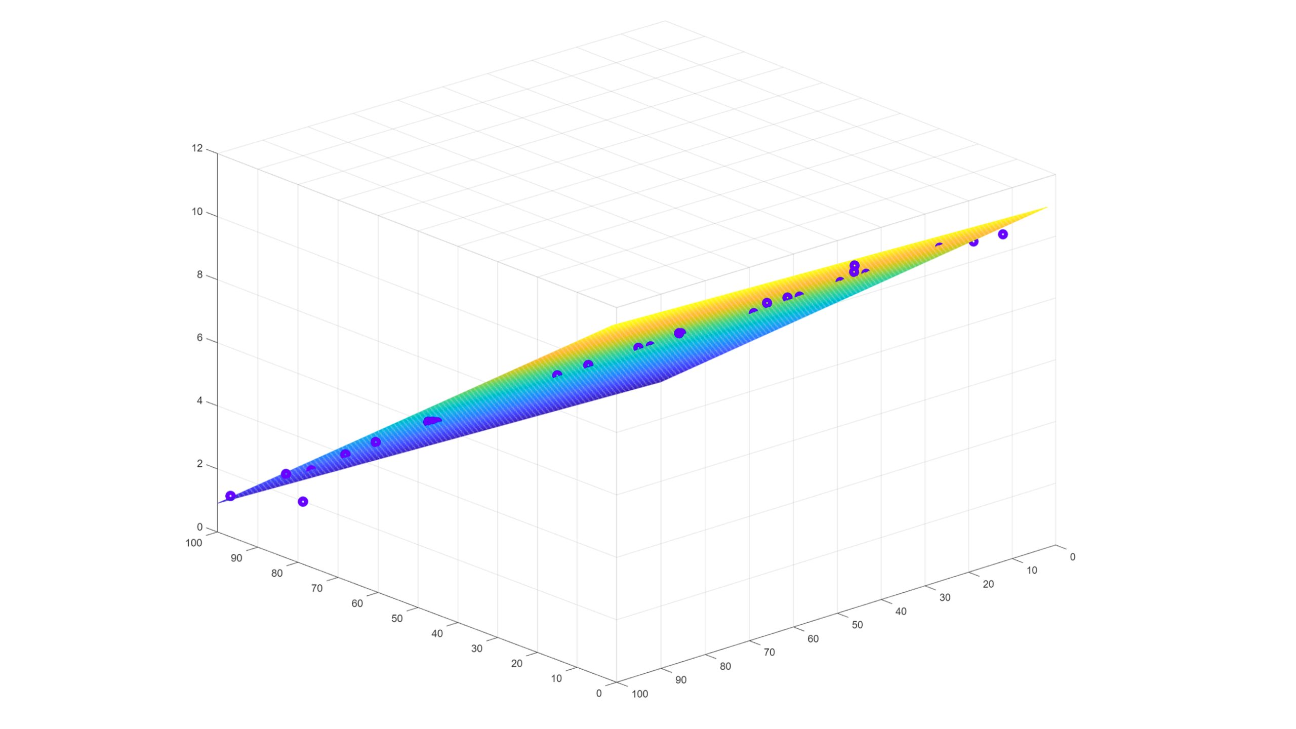
12. Plot the regression line with actual data:

Figure 82: Plotting the data on our scatterplot.

13. Define the prediction function:

Figure 83: Defining our prediction function.

14. Predicting the values based on the prediction function:

Figure 84: Predicting the values based on the prediction function.

15. Predicting values for the whole dataset:

Figure 85: Predicting the values of the whole dataset.
Figure 85: Predicting the values of the whole dataset.

16. Plotting the test data with the regression line:

Figure 86: Plotting the test data on the scatter plot with the regression line.

17. Plot the training data with the regression line:

Figure 87: Plotting the training data with the regression line.

18. Plot the complete data with regression line:

Figure 88: Plotting the data on the scatterplot with the regression line.

19. Create a data frame for actual and predicted values:

Figure 89: Actual vs. predicted values.

19. Plot the bar graph for actual and predicted values:

Figure 90: Bar graph for actual vs. predicted values.

20. Residual Sum of Square:

Figure 91: Error calculation function.

21. Calculating error:

Figure 92: Calculating the error.
Figure 92: Calculating the error.

So, that is how we can perform Simple Linear Regression from scratch with Python. Although Python libraries can perform all these calculations without diving in-depth, it is always good practice to know how these libraries perform such mathematical calculations.


Next, we will use the Scikit-learn library in Python to find the linear-best-fit regression line on the same data set. In the following code, we will see a straightforward way to calculate a simple linear regression using Scikit-learn.

Simple Linear Regression Using Scikit-learn:

  1. Import the required libraries:
Figure 93: Importing the required libraries for our Scikit implementation.

2. Read the CSV file:

Figure 94: Reading the CSV file.
Figure 94: Reading the CSV file.

3. Feature selection for regression model:

Figure 95: Feature selection.

4. Plotting the data points on a scatter plot:

Figure 96: Plotting the data points on a scatter plot.

5. Dividing data into testing and training dataset:

Figure 97: Dividing our data into test and training.

6. Training the model:

Figure 98: Training our model.

7. Predicting values for a complete dataset:

Figure 99: Predicting the values.
Figure 99: Predicting the values.

8. Predicting values for training data:

Figure 100: Predicting the values for our training dataset.
Figure 100: Predicting the values for our training dataset.

9. Predicting values for testing data:

Figure 101: Predicting the values for our testing dataset.
Figure 101: Predicting the values for our testing dataset.

10. Plotting regression line for complete data:

Figure 102: Plotting the data on the scatter plot with a regression line.

11. Plotting regression line with training data:

Figure 103: Plotting the training data on a scatter plot with a regression line.

12. Plotting regression line with testing data:

Figure 103: Plotting the testing data on our scatter plot with a regression line.
Figure 104: Plotting the testing data on our scatter plot with a regression line.

13. Create dataframe for actual and predicted data points:

Figure 105: Data frame for actual and predicted values.

14. Plotting the bar graph for actual and predicted values:

Figure 106: Plotting a bar graph for actual vs. predicted values.

15. Calculating error in prediction:

Figure 107: Calculating the error in prediction.

Here we can see that we got the same output even if we use the Scikit-learn library. Therefore we can be sure that all the calculations we performed and derivations we understood are precisely accurate.

Please note that there are other methods to calculate the prediction error, and we will try to cover them in our future tutorials.

That is all for this tutorial. We hope you enjoyed it and learned something new from it. If you have any feedback, please leave us a comment or send us an email directly. Thank you for reading!


DISCLAIMER: The views expressed in this article are those of the author(s) and do not represent the views of Carnegie Mellon University. These writings do not intend to be final products, yet rather a reflection of current thinking, along with being a catalyst for discussion and improvement.

Published via Towards AI

Resources:

Google colab implementation.

Github repository.

References:

[1] What is simple linear regression, Penn State, https://online.stat.psu.edu/stat462/node/91/

[2] scikit-learn, Getting Started, https://scikit-learn.org/

[3] SpongeBob SquarePants, Wikipedia, https://en.wikipedia.org/wiki/SpongeBob_SquarePants

[4] Deterministic: Definition and Examples, Statistics How To, https://www.statisticshowto.com/deterministic/


Feedback ↓

Sign Up for the Course
`; } else { console.error('Element with id="subscribe" not found within the page with class "home".'); } } }); // Remove duplicate text from articles /* Backup: 09/11/24 function removeDuplicateText() { const elements = document.querySelectorAll('h1, h2, h3, h4, h5, strong'); // Select the desired elements const seenTexts = new Set(); // A set to keep track of seen texts const tagCounters = {}; // Object to track instances of each tag elements.forEach(el => { const tagName = el.tagName.toLowerCase(); // Get the tag name (e.g., 'h1', 'h2', etc.) // Initialize a counter for each tag if not already done if (!tagCounters[tagName]) { tagCounters[tagName] = 0; } // Only process the first 10 elements of each tag type if (tagCounters[tagName] >= 2) { return; // Skip if the number of elements exceeds 10 } const text = el.textContent.trim(); // Get the text content const words = text.split(/\s+/); // Split the text into words if (words.length >= 4) { // Ensure at least 4 words const significantPart = words.slice(0, 5).join(' '); // Get first 5 words for matching // Check if the text (not the tag) has been seen before if (seenTexts.has(significantPart)) { // console.log('Duplicate found, removing:', el); // Log duplicate el.remove(); // Remove duplicate element } else { seenTexts.add(significantPart); // Add the text to the set } } tagCounters[tagName]++; // Increment the counter for this tag }); } removeDuplicateText(); */ // Remove duplicate text from articles function removeDuplicateText() { const elements = document.querySelectorAll('h1, h2, h3, h4, h5, strong'); // Select the desired elements const seenTexts = new Set(); // A set to keep track of seen texts const tagCounters = {}; // Object to track instances of each tag // List of classes to be excluded const excludedClasses = ['medium-author', 'post-widget-title']; elements.forEach(el => { // Skip elements with any of the excluded classes if (excludedClasses.some(cls => el.classList.contains(cls))) { return; // Skip this element if it has any of the excluded classes } const tagName = el.tagName.toLowerCase(); // Get the tag name (e.g., 'h1', 'h2', etc.) // Initialize a counter for each tag if not already done if (!tagCounters[tagName]) { tagCounters[tagName] = 0; } // Only process the first 10 elements of each tag type if (tagCounters[tagName] >= 10) { return; // Skip if the number of elements exceeds 10 } const text = el.textContent.trim(); // Get the text content const words = text.split(/\s+/); // Split the text into words if (words.length >= 4) { // Ensure at least 4 words const significantPart = words.slice(0, 5).join(' '); // Get first 5 words for matching // Check if the text (not the tag) has been seen before if (seenTexts.has(significantPart)) { // console.log('Duplicate found, removing:', el); // Log duplicate el.remove(); // Remove duplicate element } else { seenTexts.add(significantPart); // Add the text to the set } } tagCounters[tagName]++; // Increment the counter for this tag }); } removeDuplicateText(); //Remove unnecessary text in blog excerpts document.querySelectorAll('.blog p').forEach(function(paragraph) { // Replace the unwanted text pattern for each paragraph paragraph.innerHTML = paragraph.innerHTML .replace(/Author\(s\): [\w\s]+ Originally published on Towards AI\.?/g, '') // Removes 'Author(s): XYZ Originally published on Towards AI' .replace(/This member-only story is on us\. Upgrade to access all of Medium\./g, ''); // Removes 'This member-only story...' }); //Load ionic icons and cache them if ('localStorage' in window && window['localStorage'] !== null) { const cssLink = 'https://code.ionicframework.com/ionicons/2.0.1/css/ionicons.min.css'; const storedCss = localStorage.getItem('ionicons'); if (storedCss) { loadCSS(storedCss); } else { fetch(cssLink).then(response => response.text()).then(css => { localStorage.setItem('ionicons', css); loadCSS(css); }); } } function loadCSS(css) { const style = document.createElement('style'); style.innerHTML = css; document.head.appendChild(style); } //Remove elements from imported content automatically function removeStrongFromHeadings() { const elements = document.querySelectorAll('h1, h2, h3, h4, h5, h6, span'); elements.forEach(el => { const strongTags = el.querySelectorAll('strong'); strongTags.forEach(strongTag => { while (strongTag.firstChild) { strongTag.parentNode.insertBefore(strongTag.firstChild, strongTag); } strongTag.remove(); }); }); } removeStrongFromHeadings(); "use strict"; window.onload = () => { /* //This is an object for each category of subjects and in that there are kewords and link to the keywods let keywordsAndLinks = { //you can add more categories and define their keywords and add a link ds: { keywords: [ //you can add more keywords here they are detected and replaced with achor tag automatically 'data science', 'Data science', 'Data Science', 'data Science', 'DATA SCIENCE', ], //we will replace the linktext with the keyword later on in the code //you can easily change links for each category here //(include class="ml-link" and linktext) link: 'linktext', }, ml: { keywords: [ //Add more keywords 'machine learning', 'Machine learning', 'Machine Learning', 'machine Learning', 'MACHINE LEARNING', ], //Change your article link (include class="ml-link" and linktext) link: 'linktext', }, ai: { keywords: [ 'artificial intelligence', 'Artificial intelligence', 'Artificial Intelligence', 'artificial Intelligence', 'ARTIFICIAL INTELLIGENCE', ], //Change your article link (include class="ml-link" and linktext) link: 'linktext', }, nl: { keywords: [ 'NLP', 'nlp', 'natural language processing', 'Natural Language Processing', 'NATURAL LANGUAGE PROCESSING', ], //Change your article link (include class="ml-link" and linktext) link: 'linktext', }, des: { keywords: [ 'data engineering services', 'Data Engineering Services', 'DATA ENGINEERING SERVICES', ], //Change your article link (include class="ml-link" and linktext) link: 'linktext', }, td: { keywords: [ 'training data', 'Training Data', 'training Data', 'TRAINING DATA', ], //Change your article link (include class="ml-link" and linktext) link: 'linktext', }, ias: { keywords: [ 'image annotation services', 'Image annotation services', 'image Annotation services', 'image annotation Services', 'Image Annotation Services', 'IMAGE ANNOTATION SERVICES', ], //Change your article link (include class="ml-link" and linktext) link: 'linktext', }, l: { keywords: [ 'labeling', 'labelling', ], //Change your article link (include class="ml-link" and linktext) link: 'linktext', }, pbp: { keywords: [ 'previous blog posts', 'previous blog post', 'latest', ], //Change your article link (include class="ml-link" and linktext) link: 'linktext', }, mlc: { keywords: [ 'machine learning course', 'machine learning class', ], //Change your article link (include class="ml-link" and linktext) link: 'linktext', }, }; //Articles to skip let articleIdsToSkip = ['post-2651', 'post-3414', 'post-3540']; //keyword with its related achortag is recieved here along with article id function searchAndReplace(keyword, anchorTag, articleId) { //selects the h3 h4 and p tags that are inside of the article let content = document.querySelector(`#${articleId} .entry-content`); //replaces the "linktext" in achor tag with the keyword that will be searched and replaced let newLink = anchorTag.replace('linktext', keyword); //regular expression to search keyword var re = new RegExp('(' + keyword + ')', 'g'); //this replaces the keywords in h3 h4 and p tags content with achor tag content.innerHTML = content.innerHTML.replace(re, newLink); } function articleFilter(keyword, anchorTag) { //gets all the articles var articles = document.querySelectorAll('article'); //if its zero or less then there are no articles if (articles.length > 0) { for (let x = 0; x < articles.length; x++) { //articles to skip is an array in which there are ids of articles which should not get effected //if the current article's id is also in that array then do not call search and replace with its data if (!articleIdsToSkip.includes(articles[x].id)) { //search and replace is called on articles which should get effected searchAndReplace(keyword, anchorTag, articles[x].id, key); } else { console.log( `Cannot replace the keywords in article with id ${articles[x].id}` ); } } } else { console.log('No articles found.'); } } let key; //not part of script, added for (key in keywordsAndLinks) { //key is the object in keywords and links object i.e ds, ml, ai for (let i = 0; i < keywordsAndLinks[key].keywords.length; i++) { //keywordsAndLinks[key].keywords is the array of keywords for key (ds, ml, ai) //keywordsAndLinks[key].keywords[i] is the keyword and keywordsAndLinks[key].link is the link //keyword and link is sent to searchreplace where it is then replaced using regular expression and replace function articleFilter( keywordsAndLinks[key].keywords[i], keywordsAndLinks[key].link ); } } function cleanLinks() { // (making smal functions is for DRY) this function gets the links and only keeps the first 2 and from the rest removes the anchor tag and replaces it with its text function removeLinks(links) { if (links.length > 1) { for (let i = 2; i < links.length; i++) { links[i].outerHTML = links[i].textContent; } } } //arrays which will contain all the achor tags found with the class (ds-link, ml-link, ailink) in each article inserted using search and replace let dslinks; let mllinks; let ailinks; let nllinks; let deslinks; let tdlinks; let iaslinks; let llinks; let pbplinks; let mlclinks; const content = document.querySelectorAll('article'); //all articles content.forEach((c) => { //to skip the articles with specific ids if (!articleIdsToSkip.includes(c.id)) { //getting all the anchor tags in each article one by one dslinks = document.querySelectorAll(`#${c.id} .entry-content a.ds-link`); mllinks = document.querySelectorAll(`#${c.id} .entry-content a.ml-link`); ailinks = document.querySelectorAll(`#${c.id} .entry-content a.ai-link`); nllinks = document.querySelectorAll(`#${c.id} .entry-content a.ntrl-link`); deslinks = document.querySelectorAll(`#${c.id} .entry-content a.des-link`); tdlinks = document.querySelectorAll(`#${c.id} .entry-content a.td-link`); iaslinks = document.querySelectorAll(`#${c.id} .entry-content a.ias-link`); mlclinks = document.querySelectorAll(`#${c.id} .entry-content a.mlc-link`); llinks = document.querySelectorAll(`#${c.id} .entry-content a.l-link`); pbplinks = document.querySelectorAll(`#${c.id} .entry-content a.pbp-link`); //sending the anchor tags list of each article one by one to remove extra anchor tags removeLinks(dslinks); removeLinks(mllinks); removeLinks(ailinks); removeLinks(nllinks); removeLinks(deslinks); removeLinks(tdlinks); removeLinks(iaslinks); removeLinks(mlclinks); removeLinks(llinks); removeLinks(pbplinks); } }); } //To remove extra achor tags of each category (ds, ml, ai) and only have 2 of each category per article cleanLinks(); */ //Recommended Articles var ctaLinks = [ /* ' ' + '

Subscribe to our AI newsletter!

' + */ '

Take our 85+ lesson From Beginner to Advanced LLM Developer Certification: From choosing a project to deploying a working product this is the most comprehensive and practical LLM course out there!

'+ '

Towards AI has published Building LLMs for Production—our 470+ page guide to mastering LLMs with practical projects and expert insights!

' + '
' + '' + '' + '

Note: Content contains the views of the contributing authors and not Towards AI.
Disclosure: This website may contain sponsored content and affiliate links.

' + 'Discover Your Dream AI Career at Towards AI Jobs' + '

Towards AI has built a jobs board tailored specifically to Machine Learning and Data Science Jobs and Skills. Our software searches for live AI jobs each hour, labels and categorises them and makes them easily searchable. Explore over 10,000 live jobs today with Towards AI Jobs!

' + '
' + '

🔥 Recommended Articles 🔥

' + 'Why Become an LLM Developer? Launching Towards AI’s New One-Stop Conversion Course'+ 'Testing Launchpad.sh: A Container-based GPU Cloud for Inference and Fine-tuning'+ 'The Top 13 AI-Powered CRM Platforms
' + 'Top 11 AI Call Center Software for 2024
' + 'Learn Prompting 101—Prompt Engineering Course
' + 'Explore Leading Cloud Providers for GPU-Powered LLM Training
' + 'Best AI Communities for Artificial Intelligence Enthusiasts
' + 'Best Workstations for Deep Learning
' + 'Best Laptops for Deep Learning
' + 'Best Machine Learning Books
' + 'Machine Learning Algorithms
' + 'Neural Networks Tutorial
' + 'Best Public Datasets for Machine Learning
' + 'Neural Network Types
' + 'NLP Tutorial
' + 'Best Data Science Books
' + 'Monte Carlo Simulation Tutorial
' + 'Recommender System Tutorial
' + 'Linear Algebra for Deep Learning Tutorial
' + 'Google Colab Introduction
' + 'Decision Trees in Machine Learning
' + 'Principal Component Analysis (PCA) Tutorial
' + 'Linear Regression from Zero to Hero
'+ '

', /* + '

Join thousands of data leaders on the AI newsletter. It’s free, we don’t spam, and we never share your email address. Keep up to date with the latest work in AI. From research to projects and ideas. If you are building an AI startup, an AI-related product, or a service, we invite you to consider becoming a sponsor.

',*/ ]; var replaceText = { '': '', '': '', '
': '
' + ctaLinks + '
', }; Object.keys(replaceText).forEach((txtorig) => { //txtorig is the key in replacetext object const txtnew = replaceText[txtorig]; //txtnew is the value of the key in replacetext object let entryFooter = document.querySelector('article .entry-footer'); if (document.querySelectorAll('.single-post').length > 0) { //console.log('Article found.'); const text = entryFooter.innerHTML; entryFooter.innerHTML = text.replace(txtorig, txtnew); } else { // console.log('Article not found.'); //removing comment 09/04/24 } }); var css = document.createElement('style'); css.type = 'text/css'; css.innerHTML = '.post-tags { display:none !important } .article-cta a { font-size: 18px; }'; document.body.appendChild(css); //Extra //This function adds some accessibility needs to the site. function addAlly() { // In this function JQuery is replaced with vanilla javascript functions const imgCont = document.querySelector('.uw-imgcont'); imgCont.setAttribute('aria-label', 'AI news, latest developments'); imgCont.title = 'AI news, latest developments'; imgCont.rel = 'noopener'; document.querySelector('.page-mobile-menu-logo a').title = 'Towards AI Home'; document.querySelector('a.social-link').rel = 'noopener'; document.querySelector('a.uw-text').rel = 'noopener'; document.querySelector('a.uw-w-branding').rel = 'noopener'; document.querySelector('.blog h2.heading').innerHTML = 'Publication'; const popupSearch = document.querySelector$('a.btn-open-popup-search'); popupSearch.setAttribute('role', 'button'); popupSearch.title = 'Search'; const searchClose = document.querySelector('a.popup-search-close'); searchClose.setAttribute('role', 'button'); searchClose.title = 'Close search page'; // document // .querySelector('a.btn-open-popup-search') // .setAttribute( // 'href', // 'https://medium.com/towards-artificial-intelligence/search' // ); } // Add external attributes to 302 sticky and editorial links function extLink() { // Sticky 302 links, this fuction opens the link we send to Medium on a new tab and adds a "noopener" rel to them var stickyLinks = document.querySelectorAll('.grid-item.sticky a'); for (var i = 0; i < stickyLinks.length; i++) { /* stickyLinks[i].setAttribute('target', '_blank'); stickyLinks[i].setAttribute('rel', 'noopener'); */ } // Editorial 302 links, same here var editLinks = document.querySelectorAll( '.grid-item.category-editorial a' ); for (var i = 0; i < editLinks.length; i++) { editLinks[i].setAttribute('target', '_blank'); editLinks[i].setAttribute('rel', 'noopener'); } } // Add current year to copyright notices document.getElementById( 'js-current-year' ).textContent = new Date().getFullYear(); // Call functions after page load extLink(); //addAlly(); setTimeout(function() { //addAlly(); //ideally we should only need to run it once ↑ }, 5000); }; function closeCookieDialog (){ document.getElementById("cookie-consent").style.display = "none"; return false; } setTimeout ( function () { closeCookieDialog(); }, 15000); console.log(`%c 🚀🚀🚀 ███ █████ ███████ █████████ ███████████ █████████████ ███████████████ ███████ ███████ ███████ ┌───────────────────────────────────────────────────────────────────┐ │ │ │ Towards AI is looking for contributors! │ │ Join us in creating awesome AI content. │ │ Let's build the future of AI together → │ │ https://towardsai.net/contribute │ │ │ └───────────────────────────────────────────────────────────────────┘ `, `background: ; color: #00adff; font-size: large`); //Remove latest category across site document.querySelectorAll('a[rel="category tag"]').forEach(function(el) { if (el.textContent.trim() === 'Latest') { // Remove the two consecutive spaces (  ) if (el.nextSibling && el.nextSibling.nodeValue.includes('\u00A0\u00A0')) { el.nextSibling.nodeValue = ''; // Remove the spaces } el.style.display = 'none'; // Hide the element } }); // Add cross-domain measurement, anonymize IPs 'use strict'; //var ga = gtag; ga('config', 'G-9D3HKKFV1Q', 'auto', { /*'allowLinker': true,*/ 'anonymize_ip': true/*, 'linker': { 'domains': [ 'medium.com/towards-artificial-intelligence', 'datasets.towardsai.net', 'rss.towardsai.net', 'feed.towardsai.net', 'contribute.towardsai.net', 'members.towardsai.net', 'pub.towardsai.net', 'news.towardsai.net' ] } */ }); ga('send', 'pageview'); -->