


Yolo-v5 Object Detection on a custom dataset.
Last Updated on October 28, 2020 by Editorial Team
Author(s): Balakrishnakumar V
Step by step instructions to train Yolo-v5 & do Inference(from ultralytics) to count the blood cells and localize them.
I vividly remember that I tried to do an object detection model to count the RBC, WBC, and platelets on microscopic blood-smeared images using Yolo v3-v4, but I couldn’t get as much as accuracy I wanted and the model never made it to production.
Now recently I came across the release of the Yolo-v5 model from Ultralytics, which is built using PyTorch. I was a bit skeptical to start, owing to my previous failures, but after reading the manual in their Github repo, I was very confident this time and I wanted to give it a shot.
And it worked like a charm, Yolo-v5 is easy to train and easy to do inference.
So this post summarizes my hands-on experience on the Yolo-v5 model on the Blood Cell Count dataset. Let’s get started.
Ultralytics recently launched Yolo-v5. For time being, the first three versions of Yolo were created by Joseph Redmon. But the newer version has higher mean Average Precision and faster inference times than others. Along with that it’s built on top of PyTorch made the training & inference process very fast and the results are great.
So let’s break down the steps in our training process.
- Data — Preprocessing (Yolo-v5 Compatible)
- Model — Training
- Inference
And if you wish to follow along simultaneously, open up these notebooks,
Google Colab Notebook — Training and Validation: link
Google Colab Notebook — Inference: link
1. Data — Preprocessing (Yolo-v5 Compatible)
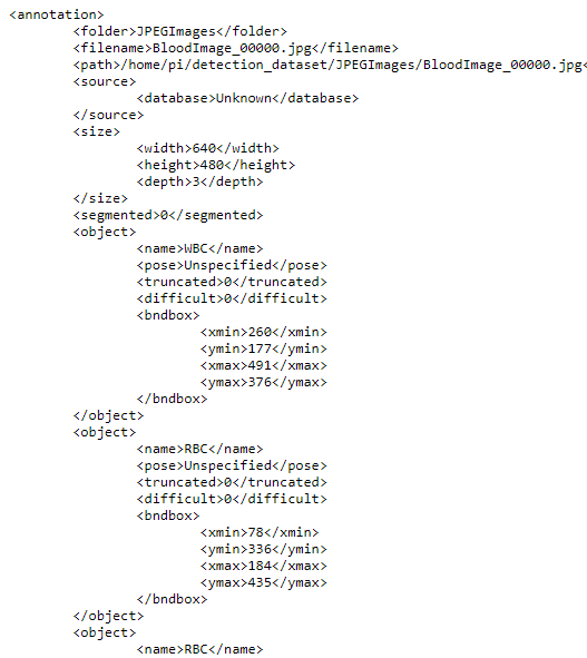
I used the dataset BCCD dataset available in Github, the dataset has blood smeared microscopic images and it’s corresponding bounding box annotations are available in an XML file.
Dataset Structure:
- BCCD
  - Annotations
    - BloodImage_00000.xml
    - BloodImage_00001.xml
    ...
- JpegImages
    - BloodImage_00001.jpg
    - BloodImage_00001.jpg
    ...
Sample Image and its annotation :
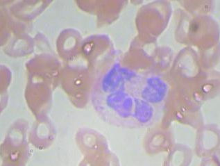
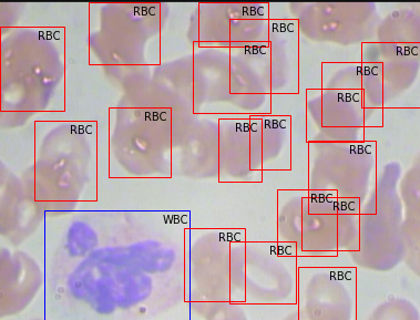
Upon mapping the annotation values as bounding boxes in the image will results like this,
But to train the Yolo-v5 model, we need to organize our dataset structure and it requires images (.jpg/.png, etc.,) and it’s corresponding labels in .txt format.
Yolo-v5 Dataset Structure:
- BCCD
  - Images
    - Train (.jpg files)
    - Valid (.jpg files)
- Labels
     - Train (.txt files)
     - Valid (.txt files)
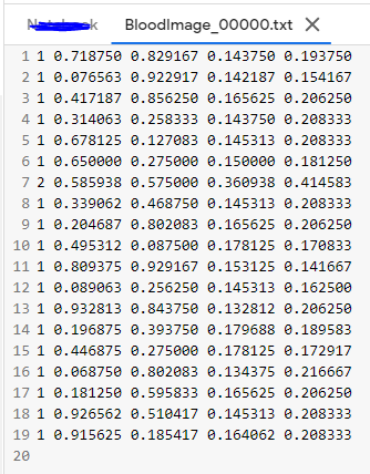
And then the format of .txt files should be :
STRUCTURE OF .txt FILE :
– One row per object.
– Each row is class x_center y_center width height format.
– Box coordinates must be in normalized xywh format (from 0–1). If your boxes are in pixels, divide x_center and width by image width, and y_center and height by image height.
– Class numbers are zero-indexed (start from 0).
An Example label with class 1 (RBC) and class 2 (WBC) along with each of their x_center, y_center, width, height (All normalized 0–1) looks like the below one.
# class x_center y_center width height #
  1     0.718    0.829    0.143 0.193
  2     0.318    0.256    0.150 0.180
  ...
So let’s see how we can pre-process our data in the above-specified structure.
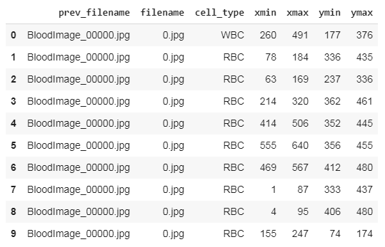
Our first step should be parsing the data from all the XML files and storing them in a data frame for further processing. Thus we run the below codes to accomplish it.
And the data frame should look like this,
After saving this file, we need to make changes to convert them into Yolo-v5 compatible format.
REQUIRED DATAFRAME STRUCTURE
- filename : contains the name of the image
- cell_type: denotes the type of the cell
- xmin: x-coordinate of the bottom left part of the image
- xmax: x-coordinate of the top right part of the image
- ymin: y-coordinate of the bottom left part of the image
- ymax: y-coordinate of the top right part of the image
- labels : Encoded cell-type (Yolo - label input-1)
- width : width of that bbox
- height : height of that bbox
- x_center : bbox center (x-axis)
- y_center : bbox center (y-axis)
- x_center_norm : x_center normalized (0-1) (Yolo - label input-2)
- y_center_norm : y_center normalized (0-1) (Yolo - label input-3)
- width_norm : width normalized (0-1) (Yolo - label input-4)
- height_norm : height normalized (0-1) (Yolo - label input-5)
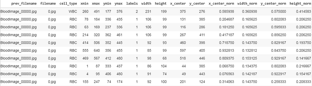
I have written some code to transform our existing data frame into the structure specified in the above snippet.
After preprocessing our data frame looks like this, here we can see there exist many rows for a single image file (For instance BloodImage_0000.jpg), now we need to collect all the (labels, x_center_norm, y_center_norm, width_norm, height_norm) values for that single image file and save it as a .txt file.
Now we split the dataset into training and validation and save the corresponding images and it’s labeled .txt files. For that, I’ve written a small piece of the code snippet.
After running the code, we should have the folder structure as we expected and ready to train the model.
No. of Training images 364
No. of Training labels 364
No. of valid images 270
No. of valid labels 270
&&
- BCCD
  - Images
    - Train (364 .jpg files)
    - Valid (270 .jpg files)
- Labels
     - Train (364 .txt files)
     - Valid (270 .txt files)
End of data pre-processing.
2. Model — Training
To start the training process, we need to clone the official Yolo-v5’s weights and config files. It’s available here.
Then install the required packages that they specified in the requirements.txt file.
bcc.yaml :
Now we need to create a Yaml file that contains the directory of training and validation, number of classes and it’s label names. Later we need to move the .yaml file into the yolov5 directory that we cloned.

## Contents inside the .yaml file
train: /content/bcc/images/train
val: /content/bcc/images/valid
nc: 3
names: ['Platelets', 'RBC', 'WBC']
model’s — YAML :
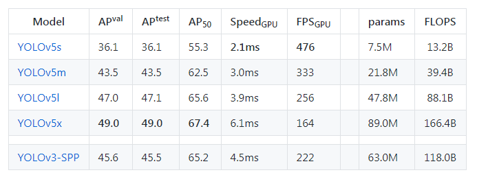
Now we need to select a model(small, medium, large, xlarge) from the ./models folder.
The figures below describe various features such as no.of parameters etc., for the available models. You can choose any model of your choice depending on the complexity of the task in hand and by default, they all are available as .yaml file inside the models’ folder from the cloned repository
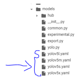
Now we need to edit the *.yaml file of the model of our choice. We just have to replace the number of classes in our case to match with the number of classes in the model’s YAML file. For simplicity, I am choosing the yolov5s.yaml for faster processing.
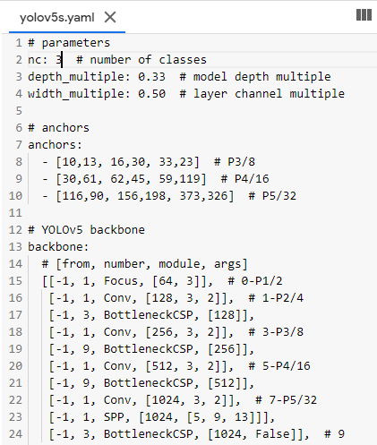
## parameters
nc: 3 # number of classes
depth_multiple: 0.33 # model depth multiple
width_multiple: 0.50 # layer channel multiple
# anchors
anchors:
- [10,13, 16,30, 33,23]  # P3/8
- [30,61, 62,45, 59,119]  # P4/16
...............
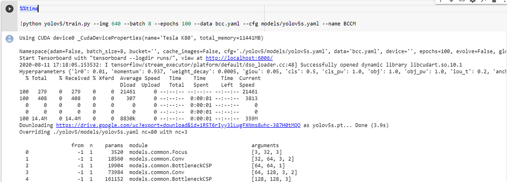
NOTE: This step is not mandatory if we didn’t replace the nc in the model’s YAML file (which I did), it will automatically override the nc value that we created before (bcc.yaml) and while training the model, you will see this line, which confirms that we don’t have to alter it.
“Overriding ./yolov5/models/yolov5s.yaml nc=80 with nc=3”
Model train parameters :
We need to configure the training parameters such as no.of epochs, batch_size, etc.,
Training Parameters
!python
- <'location of train.py file'>
- --img <'width of image'>
- --batch <'batch size'>
- --epochs <'no of epochs'>
- --data <'location of the .yaml file'>
- --cfg <'Which yolo configuration you want'>(yolov5s/yolov5m/yolov5l/yolov5x).yaml | (small, medium, large, xlarge)
- --name <'Name of the best model to save after training'>
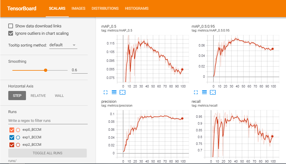
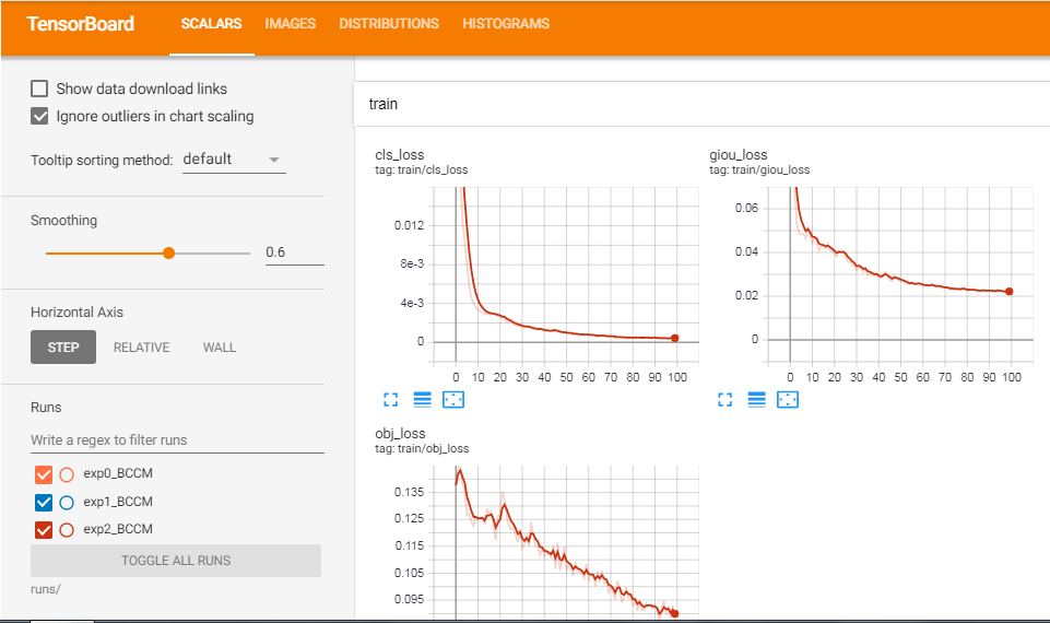
Also, we can view the logs in tensorboard if we wish.
This will initiate the training process and takes a while to complete.
I am posting some excerpts from my training process,
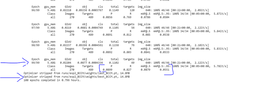
METRICS FROM TRAINING PROCESS
No.of classes, No.of images, No.of targets, Precision (P), Recall (R), mean Average Precision (map)
- Class | Images | Targets | P | R | [email protected] | [email protected]:.95: |
- all | 270 | 489 | 0.0899 | 0.827 | 0.0879 | 0.0551
So from the values of P (Precision), R (Recall), and mAP (mean Average Precision) we can know whether our model is doing well or not. Even though I have trained the model for only 100 epochs, the performance was great.
End of model training.
3. Inference
Now it’s an exciting time to test our model, to see how it makes the predictions. But we need to follow some simple steps.
Inference Parameters
Inference Parameters
!python
- <'location of detect.py file'>
- --source <'location of image/ folder to predict'>
- --weight <'location of the saved best weights'>
- --output <'location to store the outputs after prediction'>
- --img-size <'Image size of the trained model'>
(Optional)
- --conf-thres <"default=0.4", 'object confidence threshold')>
- --iou-thres <"default=0.5" , 'threshold for NMS')>
- --device <'cuda device or cpu')>
- --view-img <'display results')>
- --save-txt <'saves the bbox co-ordinates results to *.txt')>
- --classes <'filter by class: --class 0, or --class 0 2 3')>
## And there are other more customization availble, check them in the detect.py file. ##
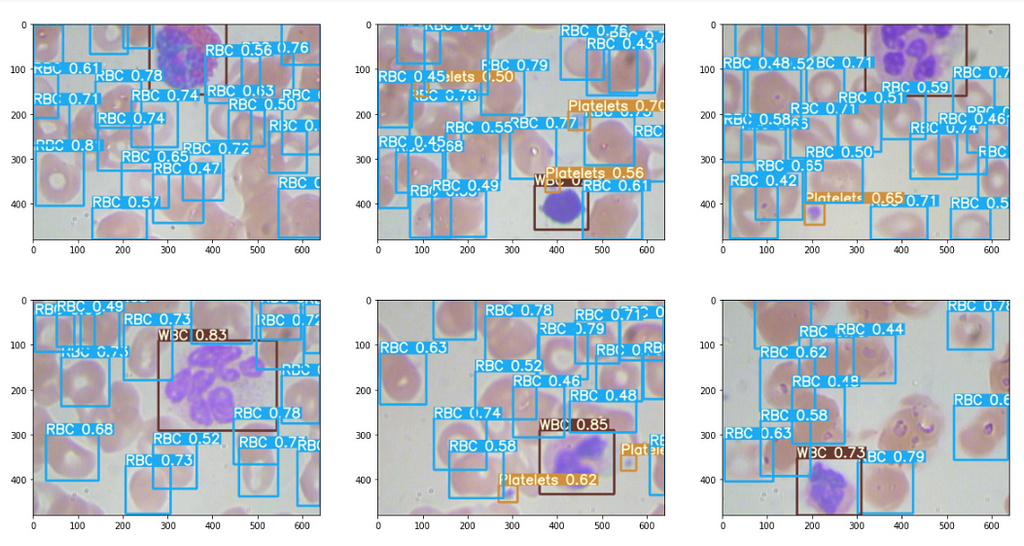
Run the below code, to make predictions on a folder/image.
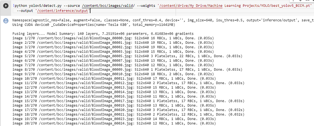
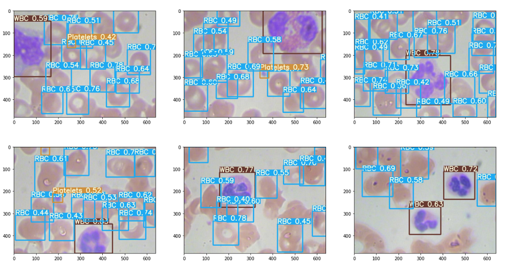
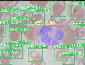
The results are good, some excerpts.
Interpret outputs from the .txt file : (Optional Read)
Also, we can save the output to a .txt file, which contains some of the input image’s bbox co-ordinates.
# class x_center_norm y_center_norm width_norm height_norm #
  1     0.718         0.829         0.143      0.193
  ...
Run the below code, to get the outputs in .txt file,
Upon successfully running the code, we can see the output are stored in the inference folder here,
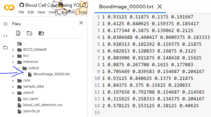
Great, now the outputs in the .txt file are in the format,
[ class x_center_norm y_center_norm width_norm height_norm ]
"we need to convert it to the form specified below"
[ class, x_min, y_min, width, height ]
[ class, X_center_norm, y_center_norm, Width_norm, Height_norm ] , we need to convert this into →[ class, x_min, y_min, width, height ] , ( Also De-normalized) to make plotting easy.
To do so, just run the below code which performs the above transformation.
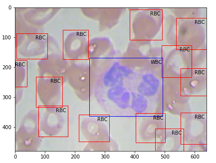
Then the output plotted image looks like this, great isn’t.
4. Moving Model to Production
Just in case, if you wish to move the model to the production or to deploy anywhere, you have to follow these steps.
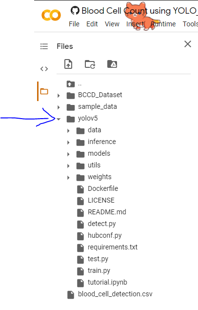
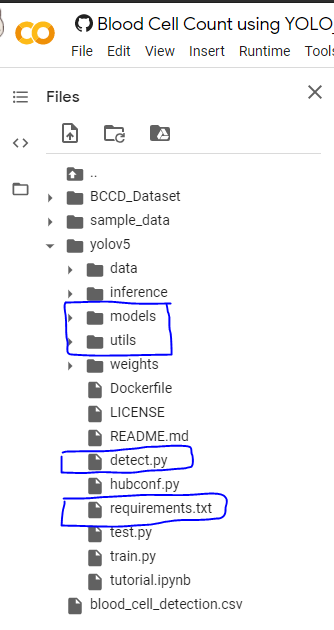
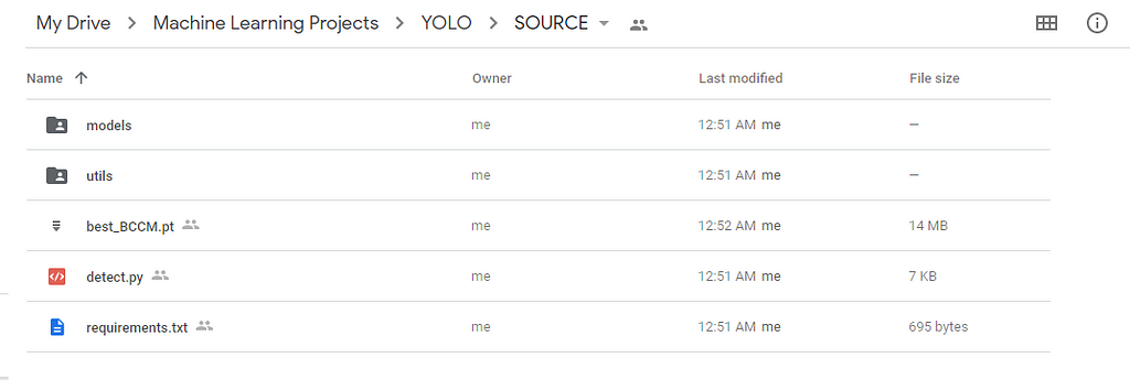
First, install the dependencies to run the yolov5, and we need some files from the yolov5 folder and add them to the python system path directory to load the utils. So copy them into some location you need and later move them wherever you need.
So in the below picture-1, I have boxed some folders and files, you can download them and keep them in a separate folder as in picture-2.
Now we need to tell the python compiler to add the above folder location into account so that when we run our programs it will load the models and functions on runtime.
In the below code snippet, on line-9, I have added the sys.path… command and in that, I have specified my folder location where I have moved those files, you can replace it with yours.
Then fire up these codes to start prediction.
And there we come to the end of this post. I hope you got some idea about how to train Yolo-v5 on other datasets you have. Let me know in the comments if you face any difficulty in training and inference.
References:
To know more about Yolo-v5 in detail, check the official Github repo.
I have trained the entire BCC model in a Colab Notebook, in case if you wish to take a look at it, it’s available in the below links.
Google Colab Notebook — Training and Validation: link
Google Colab Notebook — Inference: link
All other supporting files and notebooks are also available at my GitHub repo here: https://github.com/bala-codes/Yolo-v5_Object_Detection_Blood_Cell_Count_and_Detection
Until then, see you next time.
Article By:
BALAKRISHNAKUMAR V
Co-Founder — DeepScopy
Connect with me → LinkedIn, GitHub, Twitter, Medium

Visit us → DeepScopy
Connect with us → Twitter, LinkedIn, Medium
Yolo-v5 Object Detection on a custom dataset. was originally published in Towards AI — Multidisciplinary Science Journal on Medium, where people are continuing the conversation by highlighting and responding to this story.
Published via Towards AI
Related posts


Comment (1)
Leave a Reply to D Cancel reply
Popular posts

 for 2021")


Updates

Recent Posts


D
Hi, thank you for your post because it helps me in my project. I just want to know, since you have all your folders and files needed for production in the drive, how does the yolov5-prod.py knows where to get the files? I want to deploy the model in pi, so I just need to run the command to run the yolov5-prod.py in the terminal, to perform prediction, right? Thank you.