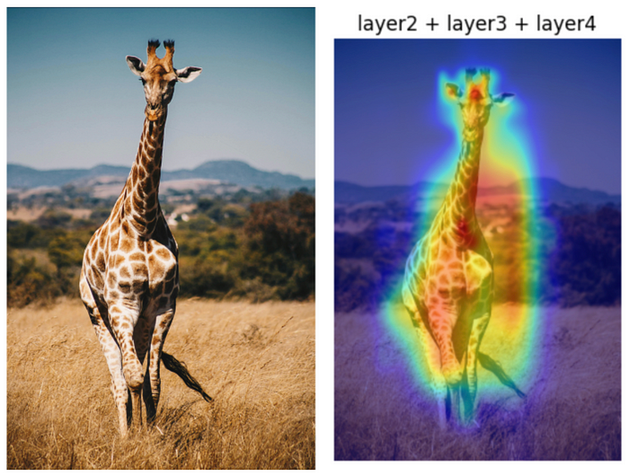
easy-explain: Explainable AI with GradCam

Author(s): Stavros Theocharis

Originally published on Towards AI.

Introduction

It’s been a while since I created this package ‘easy-explain’ and published it on Pypi. I have already written several articles on Medium about the functionality on image models using Occlusion & YoloV8 models using LRP.

GradCam is a widely used Explainable AI method that has been extensively discussed in both forums and literature. Therefore, I thought, why not include this common method in my package, but in an abstract way, so that, as my motto says, someone can use it easily!

The package has already been transformed since my previous release to make it easier for me to add a new method each time without breaking the entire structure. The logic is that each of my methods has its own class and can be called directly from the package. The plotting functionality is also included, so you only need to run a few lines of code.

So, let's read some of the theory…

What is GradCam

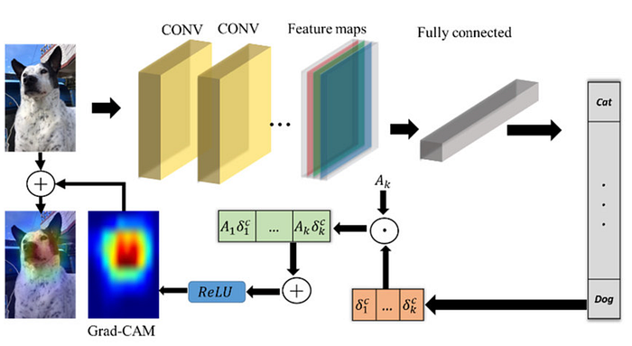
Grad-CAM, or Gradient-weighted Class Activation Mapping, introduced in this paper, is a prominent algorithm in Explainable AI (XAI). It was specifically developed for evaluation with pretrained networks like Resnet50 and VGG19. Grad-CAM can be used in image classification problems and enables us to identify the parts of an image that influenced the model’s labeling decision.

It has been widely used, for instance, in analysis where the model may have misclassified an image. The Grad-CAM technique is known for its simplicity and ease of implementation. The architecture of Grad-CAM is depicted in the image below.

In this package, we offer two different options based on the user’s needs: SmoothGradCAMpp and LayerCAM.

SmoothGradCAMpp

SmoothGradCAMpp is an extension of Grad-CAM++ (Gradient-weighted Class Activation Mapping) and integrates ideas from SmoothGrad. Grad-CAM++ itself is an improvement over Grad-CAM, designed to provide finer-grained visual explanations of CNN decisions.

The core idea of Grad-CAM++ (and by extension, SmoothGradCAMpp) is to use the gradients flowing into the final convolutional layer of the CNN to produce a heatmap that highlights the important regions in the input image for predicting the concept. SmoothGradCAMpp enhances this by averaging the maps obtained from multiple noisy versions of the input image, aiming to reduce noise and highlight salient features more effectively.

SmoothGradCAMpp is particularly useful for getting more detailed and less noisy heatmaps that indicate why a particular decision was made by the model. It’s beneficial for understanding model behavior in a specific instance.

LayerCAM

LayerCAM is a relatively newer technique that also aims to provide visual explanations for model decisions. Unlike Grad-CAM and its variants, LayerCAM can generate more detailed heatmaps by integrating features from multiple layers of CNN.

LayerCAM modifies the way of aggregating feature maps from different layers. It emphasizes the importance of each pixel by considering its influence across multiple layers, not just the final convolutional layer. This approach allows LayerCAM to highlight finer details and more relevant areas in the input image for the model’s decision.

LayerCAM is particularly useful when you want to capture the model’s attention at multiple levels of abstraction, from lower-level features to higher-level semantics. It can provide a more comprehensive view of how different layers contribute to the final decision, making it valuable for in-depth analysis of model behavior.

Key differences

• Layer Focus: SmoothGradCAMpp focuses on the final convolutional layer and uses noise reduction techniques to enhance clarity. LayerCAM aggregates information across multiple layers for a more detailed heatmap.
• Detail and Scope: LayerCAM can potentially provide more detailed insights by leveraging multiple layers, while SmoothGradCAMpp seeks to refine the clarity of heatmaps derived from a single layer.
• Noise Reduction: The integration of SmoothGrad into GradCAMpp (forming SmoothGradCAMpp) specifically aims to reduce noise in the generated heatmaps, a feature not explicitly designed into LayerCAM.
• Implementation Complexity: SmoothGradCAMpp’s methodology of adding noise and averaging might be more straightforward to implement as an extension of existing Grad-CAM++ techniques, while LayerCAM requires a more complex aggregation of features across layers.

Both methods offer valuable insights into model decisions, and the choice between them depends on the specific requirements of the explanation task, such as the need for detail, clarity, or understanding multi-layer contributions.

How to use it (Code part)

In this example, I am going to showcase the same one with the example notebooks provided inside the repo.

I will also load two different models from torchvision to demonstrate the possible uses of the package. So, let’s import the libraries. We also assume that the package has been installed via “pip install easy-explain”.

from torchvision.models import resnet50, vgg19
from torchvision.io.image import read_image
from easy_explain import CAMExplain

Now let's initialize the models to be used:

resnet50_model = resnet50(weights="ResNet50_Weights.DEFAULT").eval()
vgg19_model = vgg19(weights="VGG19_Weights.DEFAULT").eval()

We also need to apply specific transformations (resizing and normalization) to the image before passing it through the models:

trans_params = {"ImageNet_transformation":
 {"Resize": {"h": 224,"w": 224},
 "Normalize": {"mean": [0.485, 0.456, 0.406], "std": [0.229, 0.224, 0.225]}}}

And now let's get an image from Unsplash.

You can save this image to your path. My path will be as follows, inside a data folder. So, I will load it from there:

img = read_image("../data/mike-setchell-pf97TYdQlWM-unsplash.jpg")

And now… we have our new explainer!

explainer = CAMExplain(model = resnet50_model) 

You can easily initialize it! In addition, let’s convert the image to a tensor in order to pass it through the model (also applying the transformation mentioned above). The explainer has built-in functionality for such image transformation.

input_tensor = explainer.transform_image(img, trans_params["ImageNet_transformation"])

Let’s also take a look at the ResNet50 model architecture to understand the layers and identify what we would like to see through the XAI application.

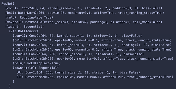
This needs to be done since each model has a different number of layers, names, etc. To determine the specific layers to analyze using Class Activation Mapping (CAM), we must inspect the model’s architecture and select the relevant layers based on our objective, such as identifying which features influence the model’s predictions at different levels.

Each model possesses unique layers, necessitating an overview of its structure to make an informed selection. By default, if no target layer is specified, the algorithm applies to the final layer of the model. For a more comprehensive visualization, multiple layer names can be included in a list.

Application of the XAI

Let’s visualise for this model some of our preference layers. We will select layers 2, 3 & 4.

explainer.generate_explanation(img, input_tensor, multiple_layers=["layer2", "layer3", "layer4"])

and this results to:

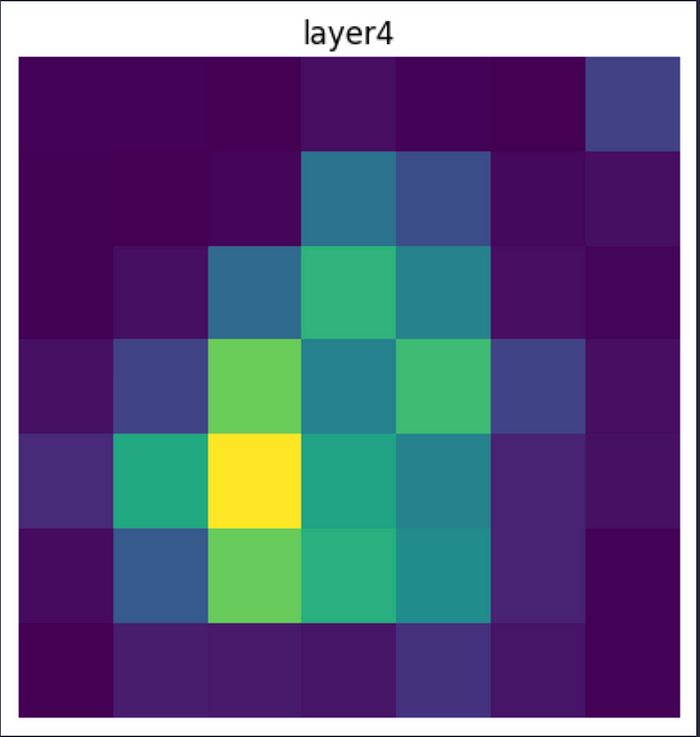
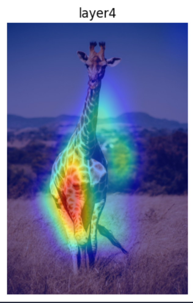
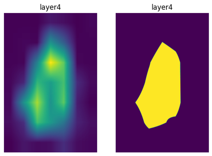
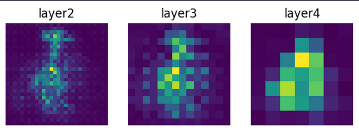
The impact of each layer on the outcome is distinct, as observed from the different layers. Every layer contributes uniquely to the final decision. Ultimately, we can view an aggregated visualization that combines the effects of all the chosen layers.

We can see that we have various visualizations of the layers. This can be very helpful in understanding how each one contributes to the final classification. These visualizations can be really useful in custom training models. In such models, the AI developer will want to see if the model behaves well and on what parts it focuses more.

Now let’s use another model (vgg model). As mentioned, each model features a unique architecture, comprising distinct layers and naming conventions for those layers.

For the ResNet50 model, GradCam was applied to its final layer by default (since None is specified), as well as an aggregated GradCam analysis for layers “layer2”, “layer3”, and “layer4”.

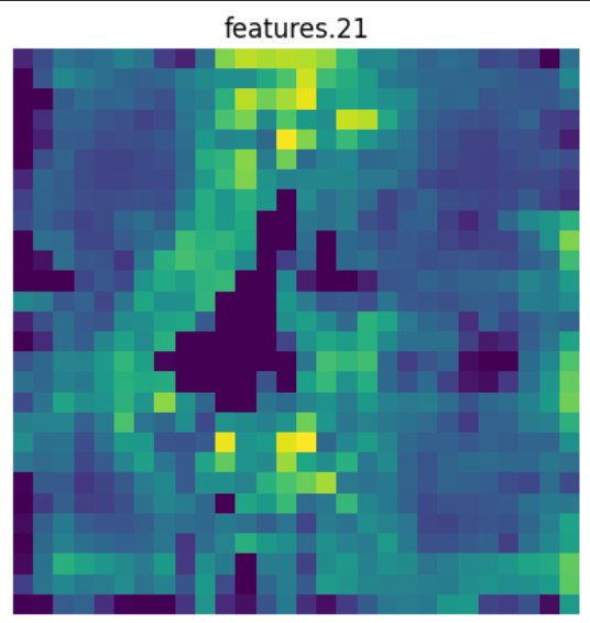
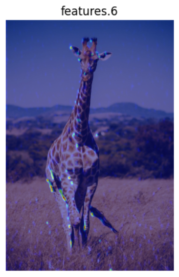
For the VGG19 model, GradCam is executed individually for each layer within the features section to also demonstrate the possible use of this XAI package.

again… a new explainer:

explainer = CAMExplain(model = vgg19_model)

Let’s have a look at the architecture again…

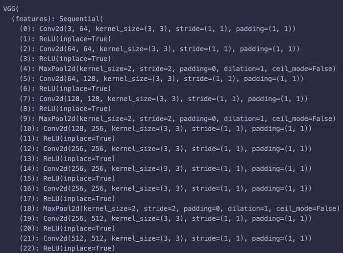
It is of course different than the previous model…

Let’s visualize for this model all the layers with features. Through these visualizations, we will be able to understand how each one of the features that the model extracts from the image behaves in order to contribute to the final result.

# Keep the features layers until the last CNN layer
features = []
features = [vgg19_model.features[x] for x in range(35)]

explainer.generate_explanation(img, input_tensor, target_layer=features)

The script mentioned above will create visualizations for all of the features identified in the model’s architecture. Below, I provide only a sample of the plots that are generated.

Conclusion

Generally, the field of explainable artificial intelligence (XAI) plays a crucial role in ensuring that artificial intelligence systems are interpretable, transparent, and reliable. By employing XAI techniques in the creation of image classification models, we can achieve a deeper comprehension of their functionality and make informed decisions regarding their application.

In this article, I showcased the new functionality of my easy-explain package. Through it, someone can easily and quickly explain and check the predictions of many known image classification models like Resnet50 or VGG19.

I encourage you to experiment with this new feature of my easy-explain package for explaining easily image models.

Possible feedback is more than welcome! If you want to contribute to the project, please read the contribution guide.

U+1F31F If you enjoyed this article, follow me on Medium to read more!

U+1F31F you can also follow me on Linkedin & Github!

References

[1] Lin, Cheng-Jian & Jhang, Jyun-Yu. (2021). Bearing Fault Diagnosis Using a Grad-CAM-Based Convolutional Neuro-Fuzzy Network. Mathematics. 9. 1502. 10.3390/math9131502.

Join thousands of data leaders on the AI newsletter. Join over 80,000 subscribers and keep up to date with the latest developments in AI. From research to projects and ideas. If you are building an AI startup, an AI-related product, or a service, we invite you to consider becoming a sponsor.

Published via Towards AI