Policy Gradient Algorithm’s Mathematics Explained with PyTorch Implementation

Author(s): Ebrahim Pichka

Originally published on Towards AI.

Table of Content

· Introduction
· Policy Gradient Method
∘ Derivation
∘ Optimization
∘ The Algorithm
· PyTorch Implementation
∘ Networks
∘ Training Loop (Main algorithm)
∘ Training Results
· Conclusion
· References

Introduction

Reinforcement Learning (RL) is a subdomain of AI that aims to enable machines to learn and improve their behavior by interacting with an environment and receiving feedback in the form of reward signals. This environment is mathematically formulated as a Markov Decision Process (MDP) where at each timestep, the agent is known to be at a certain state (s ∈ S) where it is able to take action (a ∈ A). This action results in a transition from state s to a new state (s’ ∈ S) with a certain probability from a dynamics function P(s, a, s’) and receiving a scalar reward r from a reward function R(s, a, s’). That said, MDPs can be shown by a tuple of sets (S, A, P, R, γ) in which γ ∈ (0, 1] is a discount factor for future steps’ rewards.

RL algorithms can be generally categorized into two groups i.e., value-based and policy-based methods. Value-based methods aim at estimating the expected return of the states and selecting an action in that state which results in the highest expected value, which is rather an indirect way of behaving optimally in an MDP environment. In contrast, policy-based methods try to learn and optimize a policy function, which is basically a mapping from states to actions. The Policy Gradient (PG) method [1][2] is a popular policy-based approach in RL, which directly optimizes the policy function by changing its parameters using gradient ascent.

PG has some advantages over value-based methods, especially when dealing with environments with continuous action spaces or high stochasticity. PG can also handle non-differentiable policies, making it suitable for complex scenarios. However, PG can suffer from some issues such as high variance in the gradient estimates, which can lead to slower convergence and/or instability.

In this post, we will lay out the Policy Gradient method in detail, while examining its strengths and limitations. We will discuss the intuition behind PG, how it works, and also provide a code implementation of the algorithm. I will try to cover various modifications and extensions that have been proposed to improve its performance in further posts.

Policy Gradient Method

As explained above, Policy Gradient (PG) methods are algorithms that aim to learn the optimal policy function directly in a Markov Decision Processes setting (S, A, P, R, γ). In PG, the policy π is represented by a parametric function (e.g., a neural network), so we can control its outputs by changing its parameters. The policy π maps state to actions (or probability distributions over actions).

The goal of PG is to achieve a policy that maximizes the expected cumulative rewards over a trajectory of states and actions (A.K.A. the return). Let us go through how it achieves to do so.

Derivation

So, considering we have a policy function π, parameterized by a parameter set θ. Given a state as input, The policy outputs a probability distribution over actions at each state. Knowing this, first, we need to come up with an objective/goal so that we would want to optimize our policy function’s parameters with regard to this goal.

Note that this policy function could be approximated with any function approximation technique. However, in the case of Deep RL, we consider this function to be approximated by a Neural Network (with parameter set θ) that takes states (observations) as input and outputs the distribution over actions. It could be a discrete distribution for discrete actions or a continuous distribution for continuous actions.

In general, the agent’s goal would be to obtain the maximum cumulative reward over a trajectory of interactions (state-action sequences). So, let τ denote such trajectory i.e., a state-action sequence s₀, a₀, s₁, a₁, …, sₕ, aₕ, And R(τ) denote the cumulative reward over this trajectory a.k.a the return.

It is obvious that this trajectory τ, is a random variable because of its stochasticity. This makes R(τ) to be a stochastic function as well. As we can not maximize this stochastic function directly, we would want to maximize its expectation, meaning to maximize it on average case, while taking actions with policy π: E[ R(τ); π ].

And as a refresher on probabilities, this is how to calculate a discrete expectation of a function of a random variable:

So the final objective function that we would want to maximize is rewritten as follows. Also, we will now call this objective function, the Utility Function (U).

where P(τ; θ) is the probability of trajectory τ taking place over policy parameters θ.

Note that this utility function is written as a function of θ, a set of policy parameters, because it is only the policy that controls the path of the trajectories since the environment dynamic is fixed (and usually unknown), and we would want to optimize this utility by changing and optimizing θ. Also, note that the reward series R over the trajectory is not dependent on the policy. Hence it is not dependent on the parameters θ because it is based on the environment and is only an experienced scalar value.

Optimization

Now that we have the Utility function U(θ), we would want to optimize it using a stochastic gradient-based optimization algorithm, namely Stochastic Gradient Ascent:

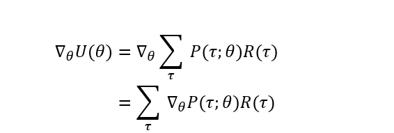
To be able to perform the parameter update, we have to compute the gradient of the Utility over θ (∇U). By attempting to do so, we get:

Note that the gradient over the summation is equal to the sum of gradients. Now we continue by applying a trick by multiplying this expression by P(τ; θ)/P(τ; θ), which equals 1. Remember from calculus that
∇f(x)/f(x) = ∇log(f(x)), so we get:

We do this trick to create a general form of expectation ‘ΣP(x)f(x)’ in the gradient, which we can later replace and estimate the expectation with the average over samples of real interaction data.

As we cannot sum over ALL possible trajectories, in a stochastic setting, we estimate this expression (∇U(θ)), by generating “m” number of random trajectories using policy parameters θ and averaging the above expectation over these m trajectories to estimate the gradient ∇U(θ):

So now we have a way of estimating the gradient with trajectory samples, but there is an issue here. this gradient causes parameters θ to change in a direction that the probability of trajectories with higher return R(τ) increases the most. However, this has a disadvantage, and that is the direction of change in the trajectory probability is highly dependent on how reward function R is designed. For example, if all transitions result in a positive reward, all trajectory probabilities would be increased and no trajectory would be penalized, and vice versa for cases with negative R.

To address this issue, it is proposed to subtract a baseline value (b) [1] from the return (i.e., change ‘R(τ)’ to ‘R(τ)-b’ ) where this baseline b should estimate how would be the return on average. This helps returns to be centralized around zero which makes trajectory probabilities that performed better than average are increased and those that didn’t are decreased. There are multiple proposed ways of calculating baseline b, among which using a neural network is one that we will use later.

Further, by decomposing the trajectory probability P(τ) into Temporal timesteps and writing it as the product of the probabilities of all ‘H’ timesteps, and also by knowing that the environment dynamics does NOT depend on the parameters θ so its gradient over θ would be 1, we can rewrite the Trajectory’s gradient w.r.t. Temporal timesteps and solely based on the policy function π:

Also, we can decompose the return R(τ) as a sum of individual timestep rewards Σrₜ. And at each timestep t, we can disregard the rewards from previous timesteps 0, … , t-1 since they are not affected by the current action aₜ (Removing terms that don’t depend on current action can lower variance). Together with incorporating the baseline, we would have the following Temporal format:

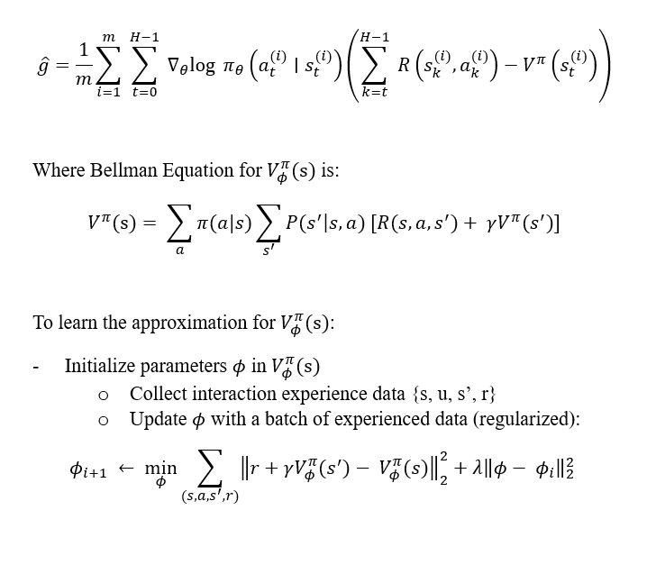
So the gradient estimate ‘g’ will be:

Finally, as a proper choice for estimation of the baseline b(sₜ), we can use expected return from state sₜ onward, which is also known as the Value function of this state V(sₜ). We will use another neural network with parameter set ϕ to approximate this value function with a bellman target using either Monte Carlo or Temporal difference learning from interaction data. the final form would be as follows:

Moreover, it is good to know that the difference between R(sₜ) and the baseline b(sₜ) is called the Advantage function A(sₜ). In some implementations, as the R(sₜ) equivalences the state-action value, also known as the Q function Q(sₜ), the advantage is written as A(sₜ) = Q(sₜ)-V(sₜ) where both Q and V can be approximated with neural networks, and maybe even with shared weights.

It is worth mentioning that when we incorporate value estimation in policy gradient methods, it is also called the Actor-Critic method, while the actor is the policy network and the critic is the value estimator network. These types of methods are highly studied nowadays due to their good performance in various benchmarks and tasks.

The Algorithm

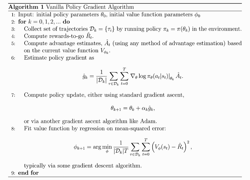
Based on the derived gradient estimator g, the Value function approximation network, and the gradient ascent update rule, the Overall algorithm to train an agent with the Vanilla (simple) Policy Gradient algorithm is as follows:

Note that in this algorithm, first, a number of state-action sequences (trajectories) are done then the updates are carried away. The policy network here is updated in an on-policy or online manner, whereas the value functions can be updated off-policy (offline) from batch-sampled data using gradient descent.

PyTorch Implementation

To implement VPG, we need the following components:

• Policy Network with probabilistic outputs to sample from. (Softmax output for discrete action space, or parameter estimations such as μ, σ output for Gaussian dist. for continuous action spaces)
• Value Network for Advantage estimation.
• Environment class with gym interface.
• Training loop

Networks

First of all, we define Policy and Value Networks as PyTorch Module classes. We are using simple Multi-layer perceptron networks for this toy task.

Importing Dependencies

# import dependencies
import torch
import torch.nn as nn
import torch.nn.functional as F
from torch.distributions import Categorical
import numpy as np
import gym
from collections import deque

Policy Net:

class PolicyNet(nn.Module):
 def __init__(self, state_dim, n_actions, n_hidden):
 super(PolicyNet, self).__init__()
 self.linear1 = nn.Linear(state_dim, n_hidden)
 self.linear2 = nn.Linear(n_hidden, n_actions)
 self.rewards, self.saved_actions = [], []

 def forward(self, x):
 out = F.relu(self.linear1(x))
 out = self.linear2(out)
 aprob = F.softmax(out, dim=1) # Softmax for categorical probabilities
 return aprob

Value Net:

class ValueNet(nn.Module):
 def __init__(self, state_dim, n_hidden):
 super(ValueNet, self).__init__()
 self.linear1 = nn.Linear(state_dim, n_hidden)
 self.linear2 = nn.Linear(n_hidden, 1)

 def forward(self, x):
 out = F.relu(self.linear1(x))
 V = self.linear2(out)
 return V

Training Loop (Main algorithm)

We will be using a simple Cartpole environment from the gym library. You can read more about this environment and its state and action spaces here.

The full algorithm is as follows:

## Vanilla Policy Gradient

# create environment
env = gym.make("CartPole-v1") # sample toy environment

# instantiate the policy and value networks
policy = PolicyNet(state_dim=env.observation_space.shape[0], n_actions=env.action_space.n, n_hidden=64)
value = ValueNet(state_dim=env.observation_space.shape[0], n_hidden=64)

# instantiate an optimizer
policy_optimizer = torch.optim.SGD(policy.parameters(), lr=2e-7)
value_optimizer = torch.optim.SGD(value.parameters(), lr=1e-7)

# initialize gamma and stats
gamma=0.99
num_episodes = 5000
returns_deq = deque(maxlen=100)
memory_buffer_deq = deque(maxlen=2000)

for n_ep in range(num_episodes):
 rewards = []
 actions = []
 states = []
 # reset environment
 state = env.reset()
 done = False

 while not done:
 # recieve action probabilities from policy function
 probs = policy(torch.tensor(state).unsqueeze(0).float())

 # sample an action from the policy distribution
 policy_prob_dist = Categorical(probs)
 action = policy_prob_dist.sample()

 # take that action in the environment
 new_state, reward, done, info = env.step(action.item())

 # store state, action and reward
 states.append(state)
 actions.append(action)
 rewards.append(reward)

 memory_buffer_deq.append((state, reward, new_state))

 state = new_state

 ### UPDATE POLICY NET ###
 rewards = np.array(rewards)
 # calculate rewards-to-go
 R = torch.tensor([np.sum(rewards[i:]*(gamma**np.array(range(i, len(rewards))))) for i in range(len(rewards))])

 # cast states and actions to tensors
 states = torch.tensor(states).float()
 actions = torch.tensor(actions)

 # calculate baseline V(s)
 with torch.no_grad():
 baseline = value(states)

 # calculate utility func
 probs = policy(states)
 sampler = Categorical(probs)
 log_probs = - sampler.log_prob(actions) # "-" is because we are doing gradient ascent
 utility = torch.sum(log_probs * (R-baseline)) # loss that when differentiated with autograd gives the gradient of J(θ)
 
 # update policy weights
 policy_optimizer.zero_grad()
 utility.backward()
 policy_optimizer.step()
 
 ########################
 ### UPDATE VALUE NET ###

 # getting batch experience data 
 batch_experience = random.sample(list(memory_buffer_deq), min(256, len(memory_buffer_deq)))
 state_batch = torch.tensor([exp[0] for exp in batch_experience])
 reward_batch = torch.tensor([exp[1] for exp in batch_experience]).view(-1,1)
 new_state_batch = torch.tensor([exp[2] for exp in batch_experience])


 with torch.no_grad():
 target = reward_batch + gamma*value(new_state_batch)
 current_state_value = value(new_state_batch)

 value_loss = torch.nn.functional.mse_loss(current_state_value, target)
 # update value weights
 value_optimizer.zero_grad()
 value_loss.backward()
 value_optimizer.step()

 ########################

 # calculate average return and print it out
 returns_deq.append(np.sum(rewards))
 print("Episode: {:6d}\tAvg. Return: {:6.2f}".format(n_ep, np.mean(returns_deq)))

# close environment
env.close()

Training Results

After training the agent with the VPG for 4000 episodes, we get the following results:

It is worth mentioning that vanilla PG suffers from two major limitations:

1. It is highly sensitive to hyperparameters configuration such as gamma, learning rate, memory size, etc.
2. It is highly prone to overshooting in the policy parameter space, which makes the learning so noisy and fragile. Sometimes the agent might take a step in the parameter space into a very suboptimal area where it would not be able to recover again.

The second issue is addressed in some further variants of the PG algorithm, which I will try to cover in future posts.

An illustration of a fully trained agent controlling the Cartpole environment is shown here:

The full code of this implementation is available at this GitHub repository.

GitHub – ebrahimpichka/vanilla-pg: Simple PyTorch implementation of the Vanilla Policy Gradient…

You can't perform that action at this time. You signed in with another tab or window. You signed out in another tab or…

github.com

Conclusion

In conclusion, we have explored the Policy Gradient (PG) algorithm, a powerful approach in Reinforcement Learning (RL) that directly learns the optimal policy. Throughout this blog post, we have provided a step-by-step explanation of the PG algorithm and its implementation. We started by understanding the fundamental concept of RL and the difference between value-based and policy-based methods. We then delved into the details of PG, highlighting its objective of maximizing the expected cumulative reward by updating the policy parameters using gradient ascent. We discussed the Vanilla PG algorithm as a common implementation of PG, where we compute the gradient of the log-probability of actions and update the policy using policy gradients. Additionally, we explored the Actor-Critic method, which combines a policy network and a value function to improve convergence. While PG offers advantages in handling continuous action spaces and non-differentiable policies, it may suffer from high variance. Nevertheless, techniques like baselines and variance reduction methods can be employed to address these challenges. By grasping the intricacies of PG, you are now equipped with a valuable tool to tackle RL problems and design intelligent systems that learn and adapt through interactions with their environments.

References

[1] — Williams, R. J. (1992). Simple statistical gradient-following algorithms for connectionist reinforcement learning. Machine Learning 8:229–256.
[2] — Sutton, R. S., McAllester, D. A., Singh, S. P., Mansour, Y., et al. Policy gradient methods for reinforcement learning with function approximation. In Proc. Advances in Neural Information Processing Systems (NIPS), volume 99, pp. 1057–1063. Citeseer, 1999.
[3] — course lectures from UC Berkeley: Deep Reinforcement Learning Bootcamp
[4] — spinningup.openai.com/en/latest/algorithms/vpg.html
[5] — Richard S. Sutton and Andrew G. Barto, Reinforcement Learning: An Introduction (second edition), The MIT Press [PDF]

Join thousands of data leaders on the AI newsletter. Join over 80,000 subscribers and keep up to date with the latest developments in AI. From research to projects and ideas. If you are building an AI startup, an AI-related product, or a service, we invite you to consider becoming a sponsor.

Published via Towards AI