Can Machine Learning Outperform Statistical Models for Time Series Forecasting?

Author(s): Satyajit Chaudhuri

Originally published on Towards AI.

The role of Time Series Forecasting is very important in areas like finance, manufacturing, health, weather studies, and social sciences. These­ fields rely on these predictions to guess future needs and sale numbers. This helps them fine-tune their stock, boost the efficiency of their supply chain. It allows them to make smart choices in financial, marketing, and risk-related areas. Hence, precise forecasting is a must for businesses to adapt to market shifts and stay ahead of competitors.

People often pick standard models like ARIMA (Auto Regressive Integrated Moving Average), Exponential Smoothing, and Seasonal Decomposition of Time Series (STL) for time series analysis. They’re good because they’re easy to understand, sturdy against data assumptions, and based on strong theory. This is why they’re top choices for future predictions.

As machine learning advances, we see a big increase in their use for predicting time series data. Tools like bagging and boosting stand out because they show great ability to spot tricky patterns and unusual links in time series data. Their unique feature is learning directly from raw data. They can deal with massive amounts of data and make accurate guesses.

The following article is an experimental study that uses both statistical forecasts and machine learning-based forecasts to predict the future for a practical use case. The study then proceeds to compare the forecasts based on certain accuracy metrics in order to judge if the machine learning models can give competition to their traditional counterparts.

Deep Learning models like LSTM, GRU, and Prophet are quite popular in the machine learning space. These models are often categorized as “black-box” models as their internal workings are not very transparent due to the intricate nature of neural networks. They can achieve impressive predictive performance, but understanding how they arrive at their predictions can be challenging and hence they are out of scope in this study.

The Forecasting Tool-kit

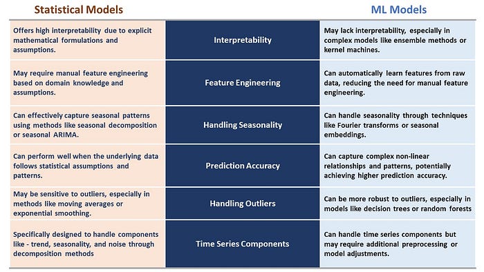
Statistical forecasting algorithms like ARIMA and ETS have been the champions in the field of time series forecasting. Libraries like pmdarima and statsforecast have performed quite well in various practical and industrial use cases. However, new and advanced machine learning models are taking the stage due to their ability to learn complex patterns from the raw data. Let’s briefly observe the differences between these algorithms.

Let’s Ensemble!

The machine learning models that we are going to explore in this study are based on the ensemble principle. Ensemble models are a machine learning approach to combine multiple other models in the forecasting process. These models are referred to as base estimators. Thus, in place of an individual model, the ensemble models use a collection of models for making forecasts.

Ensemble uses two methods:

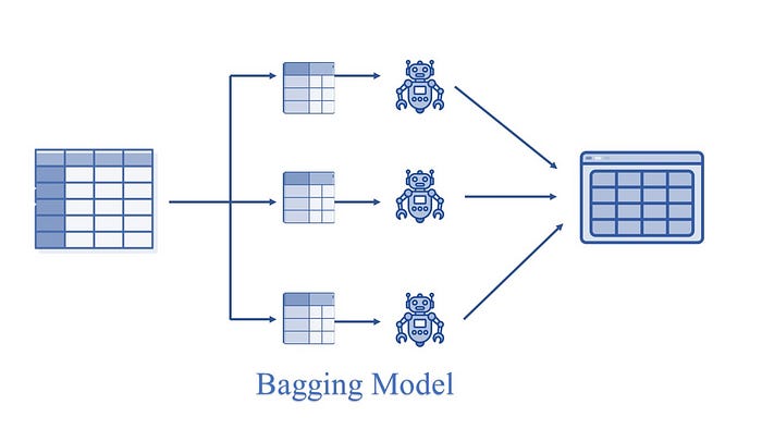
Bagging: It creates a different training subset from sample training data with replacement and the final output is based on majority voting, e,g., Random Forest.

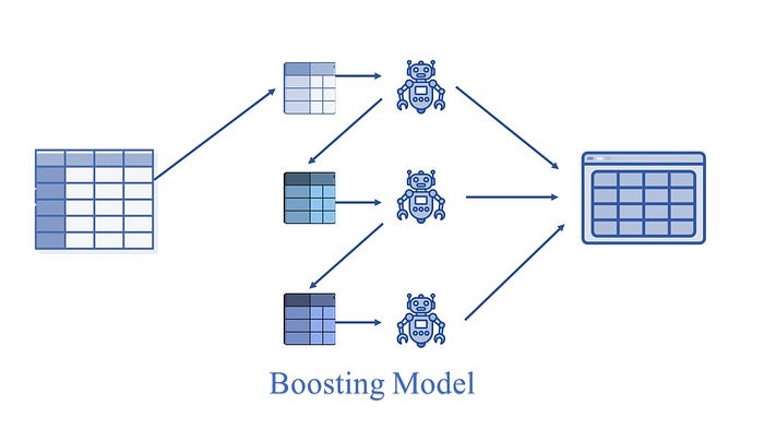
Boosting: It combines the weak learners into strong learners by creating a sequential models such that the final model has the highest accuracy.
e.g., LGBM, XGB etc.

We will not be going into the finer details of these algorithms as it is assumed that the reader has a working knowledge of Machine Learning Principles.

Data Analysis

Now let us get into the experiment part:

The dataset used in this study can be found here.

Let’s install the libraries first.

#Install statsforecast
!pip install statsforecast

#Install mlforecast. 
#This will also install collected packages: window-ops, utilsforecast, mlforecast
!pip install mlforecast

#Install pmdarima
!pip install pmdarima

The StatsForecast and MLForecast packages used in this study are designed by the NIXTLA team. Further details about them can be found here.

Now let’s import the libraries needed for this study.

import os
import pandas as pd
import seaborn as sns
import matplotlib.pyplot as plt
from statsmodels.tsa.seasonal import seasonal_decompose
from statsmodels.tsa.stattools import adfuller
from statsforecast import StatsForecast
from pmdarima import auto_arima
from statsforecast.models import AutoARIMA
from statsmodels.tsa.holtwinters import ExponentialSmoothing
from mlforecast import MLForecast
from mlforecast.target_transforms import Differences
from numba import njit
from window_ops.expanding import expanding_mean
from window_ops.rolling import rolling_mean
import lightgbm as lgb
import xgboost as xgb
from sklearn.linear_model import LinearRegression
from sklearn.ensemble import RandomForestRegressor

Let’s read the data and visualize it.

file_path = "AirPassengers.csv"
df = pd.read_csv(file_path)
df['Month'] = pd.to_datetime(df['Month'])
df = df.set_index('Month').resample('MS').mean()
df = df.interpolate() #to interpolate and fill missing values
df.reset_index(inplace=True)
print(df.head())

Let’s visualize the dataset.

sns.set(style="darkgrid")
plt.figure(figsize=(10, 6))
sns.lineplot(x="Month", y='#Passengers', data=df, color='#ff9f9b')
plt.title('Monthly Sales Over Time')
plt.xlabel('Month')
plt.ylabel('#Passengers')
plt.show()

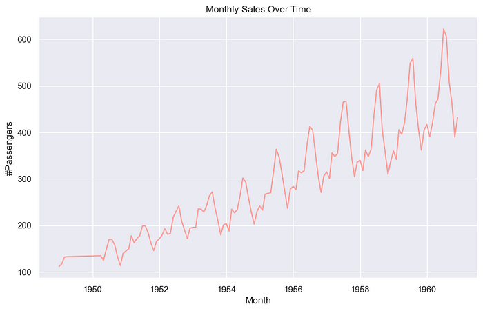
Now Let’s do the seasonal decomposition for this data.

result = seasonal_decompose(df['#Passengers'], model='additive')

fig, (ax1, ax2, ax3, ax4) = plt.subplots(4, 1, figsize=(10, 12))

result.observed.plot(ax=ax1, color="blue")
ax1.set_ylabel('Observed')

result.trend.plot(ax=ax2, color='blue')
ax2.set_ylabel('Trend')

result.seasonal.plot(ax=ax3, color='blue')
ax3.set_ylabel('Seasonal')

result.resid.plot(ax=ax4, color='blue')
ax4.set_ylabel('Residual')

plt.tight_layout()
plt.show()

Model Building

Now let’s build the Statistical and Machine Learning Models.

#Train-Test Split
train_size = int(len(df) * 0.8)
train, test = df.iloc[:train_size], df.iloc[train_size:]

print(f'Train set size: {len(train)}')
print(f'Test set size: {len(test)}')

Forecasting using pmdarima

pmdarima_model = auto_arima(train['#Passengers'], seasonal=True, m=12)
pmdarima_forecast = pmdarima_model.predict(n_periods=len(test))
pmdarima_forecast_df = pd.DataFrame({'Date': test["Month"],
 'PMDARIMA_Forecast': pmdarima_forecast})

Forecasting using Exponential Smoothening

ets_model = ExponentialSmoothing(train['#Passengers'], 
 seasonal='add', seasonal_periods=12).fit()

ets_forecast = ets_model.forecast(steps=len(test))
ets_forecast_df = pd.DataFrame({'Date': test["Month"],
 'ETS_Forecast': ets_forecast})

Forecasting using StatsForecast Library

train_ = pd.DataFrame({'unique_id':[1]*len(train),
 'ds': train["Month"], "y":train['#Passengers']})

test_ = pd.DataFrame({'unique_id':[1]*len(test),
 'ds': test["Month"], "y":test['#Passengers']})

sf_forecast = StatsForecast(models = [AutoARIMA(season_length = 12)],freq = 'MS')

sf_forecast.fit(train_)
sf_prediction = sf_forecast.predict(h=len(test))
sf_prediction.rename(columns={'ds': 'Month'}, inplace=True)

Forecasting using MLForecast Library — Linear Regression, Random Forest Regression, Light GBM Regression and Extreme Gradient Boosting Regression.

models = [LinearRegression(),
 lgb.LGBMRegressor(verbosity=-1),
 xgb.XGBRegressor(),
 RandomForestRegressor(random_state=0),
]
@njit
def rolling_mean_3(x):
 return rolling_mean(x, window_size=3)
@njit
def rolling_mean_6(x):
 return rolling_mean(x, window_size=6)

fcst = MLForecast(
 models=models,
 freq='MS',
 lags=[1,3,5,7,12],
 lag_transforms={
 1: [expanding_mean],
 3: [rolling_mean_3, rolling_mean_6],
 5: [rolling_mean_3, rolling_mean_6],
 7: [rolling_mean_3, rolling_mean_6],
 12: [rolling_mean_3, rolling_mean_6],
 },
 date_features=['year', 'month', 'day', 'quarter'],
 target_transforms=[Differences([1])])
fcst.fit(train_)
ml_prediction = fcst.predict(len(test_))
ml_prediction.rename(columns={'ds': 'Month'}, inplace=True)

Performance Evaluation and Comparison

Now let’s combine the forecasts into a single dataframe and compare them based on accuracy metrices.

fcst_result = test.copy()
fcst_result.set_index("Month", inplace=True)
fcst_result["AutoARIMA_fcst"]=sf_prediction["AutoARIMA"].values
fcst_result["LinearRegression_fcst"]=ml_prediction["LinearRegression"].values
fcst_result["LGBM_fcst"]=ml_prediction["LGBMRegressor"].values
fcst_result["XGB_fcst"]=ml_prediction["XGBRegressor"].values
fcst_result["RandomForest_fcst"]=ml_prediction["RandomForestRegressor"].values
print(fcst_result.head())

Now let’s calculate the accuracy metrices to compare the performance of this forecasting algorithms. You can read more about these metrices and their usage here.

#Defining a function to calculate the error metrices
def calculate_error_metrics(actual_values, predicted_values):
 actual_values = np.array(actual_values)
 predicted_values = np.array(predicted_values)

 metrics_dict = {
 'MAE': np.mean(np.abs(actual_values - predicted_values)),
 'RMSE': np.sqrt(np.mean((actual_values - predicted_values)**2)),
 'MAPE': np.mean(np.abs((actual_values - predicted_values) / actual_values)) * 100,
 'SMAPE': 100 * np.mean(2 * np.abs(predicted_values - actual_values) / (np.abs(predicted_values) + np.abs(actual_values))),
 'MdAPE': np.median(np.abs((actual_values - predicted_values) / actual_values)) * 100,
 'GMRAE': np.exp(np.mean(np.log(np.abs(actual_values - predicted_values) / actual_values)))
 }

 result_df = pd.DataFrame(list(metrics_dict.items()), columns=['Metric', 'Value'])
 return result_df


actuals = fcst_result['#Passengers']


error_metrics_dict = {}


for col in result.columns[2:]: # Exclude 'index' and '#Passengers'
 predicted_values = fcst_result[col]
 error_metrics_dict[col] = calculate_error_metrics(actuals, predicted_values)['Value'].values # Extracting 'Value' column


error_metrics_df = pd.DataFrame(error_metrics_dict)
error_metrics_df.insert(0, 'Metric', calculate_error_metrics(actuals, actuals)['Metric'].values) # Adding 'Metric' column
print(error_metrics_df)

Let’s also plot the actuals against each of this forecasts.

sns.set(style="darkgrid")

for col in result.columns[1:]:
 plt.figure(figsize=(10, 6)) 
 plt.plot(result.index, result['#Passengers'], label='#Passengers', color='green')
 plt.plot(result.index, result[col], label=col, color='blue')
 plt.title(f'Actuals vs {col}')
 plt.xlabel('Month')
 plt.ylabel('Values')
 plt.legend()
 plt.show()

From the error metrics we can see that:

1. Random Forecast Regression gives the lowest value for all the metrics, including RMSE & MAPE. It outperforms the traditional Statistical Models, which is quite an interesting finding of this research.
2. The Boosting algorithms — Light GBM and XGBoost Regression also give superior performance to the statistical models like Exponential Smoothing in terms of MAPE, RMSE, and MAE.
3. The performance of the MLforecast models like XGB and LGBM are also satisfactory in the sense that their accuracy metrics are in line with that of the statistical models.

Concluding Remarks

Whether Machine Learning Models can outperform statistical models for time series forecasting is a subject of ongoing debate. Both approaches demonstrate their own strengths and weaknesses. The model performance will be dependent on factors like characteristics of the data — seasonality, trend and residuals, the specific forecasting task, the model hyperparameters, computational resources, interpretability requirements and the trade-offs between simplicity and accuracy.

It is well known that statistical models are effective for capturing the linear trends, seasonal patterns, and autocorrelation present in time series data. Also machine learning models are popular due to their ability to capture complex non-linear relationships and patterns within data.

This research has well established that the machine learning models have a fair competitive chance against the established statistical models. Models like Random Forest, XGB, and LGBM have given quite satisfactory forecasts, and Random Forests have also outperformed AutoARIMA and ETS for this popular benchmark dataset.

While incorporating this model into your forecasting toolkit, it should be kept in mind that the input features to the models play a significant part, and this needs to be fine-tuned. And with efficient fine-tuning, it can be concluded that machine learning models can very well fit into the forecasting toolkit.

Disclaimer: All the images used in this article are created or generated by the author.

Join thousands of data leaders on the AI newsletter. Join over 80,000 subscribers and keep up to date with the latest developments in AI. From research to projects and ideas. If you are building an AI startup, an AI-related product, or a service, we invite you to consider becoming a sponsor.

Published via Towards AI