Understanding Machine Learning Performance Metrics

Author(s): Pranay Rishith

Originally published on Towards AI.

Evaluating the Effectiveness of Your Models

I’m sure you’re familiar with machine learning, so let’s not discuss it further. There are several types of machine learning, such as supervised and unsupervised learning. Let’s focus on supervised learning.

Supervised learning involves training a computer with labeled data in order to predict new data points. It is further divided into two subcategories: regression and classification. Each has its own performance metrics.

Classification

Classification is a supervised learning algorithm, which means that the model is trained using labeled data to predict the class to which a given data point belongs. The dependent variable is categorical, meaning it has two or more classes.

Examples of classification include determining whether an email is spam or not.

Let’s discuss some performance metrics of classification.

Confusion Matrix

Seeing the name don’t get confused U+1F602. In machine learning, a classification problem is used to define something as either 0 or 1. But how do we find out if the model has correctly classified something? This is where the confusion matrix comes into play. A confusion matrix is a [0,1] matrix or table which explains comprehensively how good our model is.

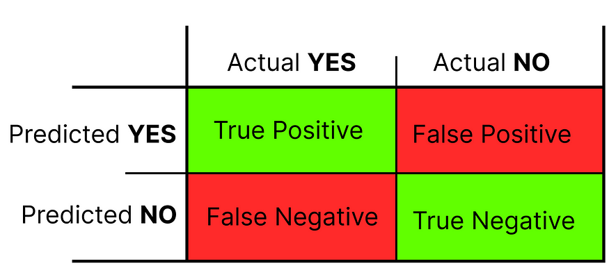
The figure above is a confusion matrix. Let’s break it down. This matrix has two-row headings (Predicted YES and Predicted NO) and two-column headings (Actual YES and Actual NO). The Actual heading refers to the classes defined in the dataset, while the Predicted refers to the classes predicted.

Let’s take an example and, if possible, use it throughout the article.

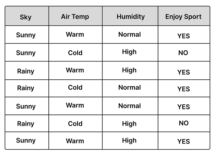
The data is provided solely for illustrative purposes.

The table above displays four features, with Enjoy Sport as the dependent variable to be predicted. The Enjoy Sport column is the actual column in the confusion matrix, while the predicted values are placed in the predicted row.

As you can see, a confusion matrix has four values: true positives, true negatives, false positives, and false negatives. Let’s dive deeper.

True Positive

• This value indicates the number of data points the model correctly predicted as positive when compared to the actual values. In other words, the model predicted “YES” when the actual value was “YES”.

True Negative

• This value indicates the number of data points the model correctly predicted as negative when compared to the actual values. In other words, the model predicted “NO” when the actual value was “NO”.

False Positive (ERROR)

• This value indicates the number of data points the model has incorrectly predicted as negative when compared to the actual values. For example, the model predicted “NO” when the actual value was “YES”.

False Negative (ERROR)

• This value indicates the number of data points the model has incorrectly predicted as positive when compared to the actual values. For example, the model predicted “YES” when the actual value was “NO”.

The Confusion Matrix can provide insight into the quality of the model by showing how many correct and incorrect predictions it has made. It is particularly useful for assessing the following few performance metrics.

Accuracy

Accuracy is a metric that measures how well a model predicts the correct output for given data points. It is calculated by dividing the number of correct predictions made by the model by the total number of predictions made.

For example, consider the above example: accuracy is the percentage of correct predictions, regardless of whether they are “yes” or “no,” out of the total number of predictions.

Mathematically, accuracy is calculated as follows:

• Accuracy = (correct predictions) / (total number of predictions)

For example, if the total number of predictions is 100 and the model predicts 73 correctly, then the accuracy is 73%.

If we use a confusion matrix, then we can get a much more simple and significant formula:

Precision

This is a metric that defines how accurately the model has predicted with respect to a specific class. It is calculated by dividing the number of true positives by the total number of positive predictions made.

It is calculated as,

where,

• TP refers to the number of values where the model predicted YES, and the actual value was also YES.
• FP is the number of values where the model predicted YES, but the actual value was NO.

Recall

This measure defines how many positive classes the model can correctly identify. It is calculated by dividing the number of true positive predictions by the total number of actual positives.

It is calculated as,

where,

• TP: the number of values where the model predicted YES and the actual value was also YES.
• FN: the number of values where the model predicted NO, but the actual value was YES.

F1 score

This metric combines recall and precision and is calculated as the harmonic mean of the two. It is mainly used to evaluate the effectiveness of a classification model.

This can be calculated as,

F1 scores range from 0 to 1, with higher values indicating better performance. A perfect score is achieved when both recall and precision are 1.

Regression

Regression is a supervised learning algorithm, which means that the model is trained using labeled data to predict a value. The dependent variable is continuous, meaning it is a real number.

Examples of regression include determining the price of a house in the US (which is a real number).

Let’s discuss some performance metrics of regression.

Mean Squared Error (MSE)

This is the most commonly used loss function for regression models. It is calculated by taking the average of the squared differences between the predicted and actual values.

The formula is as follows,

where,

• n is the number of data points
• y_pred is the predicted value
• y is the actual value

The Mean Squared Error (MSE) is a non-negative value. A lower value indicates a better fit of the regression model; values close to 0 indicate the best fit, while values of 1 or more indicate a poor fit.

MSE is most often used as a loss function when training a machine learning model for regression tasks, as it can be minimized using gradient descent.

Mean Absolute Error (MAE)

This is a metric used to evaluate the performance of a model in regression tasks. It is calculated by taking the average of the absolute differences between the predicted and actual values. The absolute error of a single data point is calculated as the absolute difference between the predicted and actual values.

The formula is as follows:

where,

• n is the number of data points
• y_pred is the predicted value
• y is the actual value

The Mean Absolute Error (MAE) is a non-negative value. The lower the value, the better the regression model. If the MAE is close to 0, it indicates the best fit; values of 1 or more indicate a poor fit.

Root Mean Squared Error (RMSE)

This metric is used to evaluate the performance of a regression model. It is calculated by taking the square root of the average of the squared differences between the predicted and actual values.

The Mean Squared Error (MSE) is the average of the squared differences between the predicted and actual values. The Root Mean Squared Error (RMSE) is the square root of this value.

The formula is as follows,

where,

• n is the number of data points
• y_pred is the predicted value
• y is the actual value

The Root Mean Squared Error (RMSE) is a non-negative value. A lower RMSE indicates a better fit of the regression model; values close to 0 indicate the best fit, while values of 1 or more indicate a poor fit. Compared to the Mean Squared Error (MSE), RMSE tends to have smaller values, making it easier to interpret.

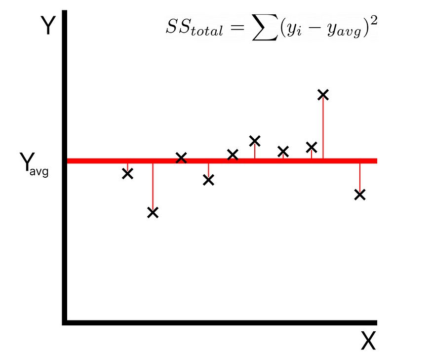
R-Squared (R²)

R-squared is a statistical measure that indicates how well a regression model fits the data. An ideal R-squared value is 1, meaning the model fits perfectly. The closer the R-squared value is to 1, the better the model fits the data.

The total sum of squares is calculated by the summation of squares of perpendicular distance between data points and the average line.

The residual sum of squares (SSres) is calculated by summing the squares of the perpendicular distances between data points and the best-fitted line.

R-Squared’s formula:

Where,

• SSres is the residual sum of squares
• SStot is the total sum of squares.

The goodness of fit of regression models can be evaluated using the R-square method. The higher the value of the R-square, the better the model is.

I hope I’ve helped you understand some fundamental concepts about performance measurements. If you enjoy this content, giving it some clapsU+1F44F will give me a little extra motivation.

You can reach me at:

LinkedIn: https://www.linkedin.com/in/pranay16/

Github: https://github.com/pranayrishith16

Join thousands of data leaders on the AI newsletter. Join over 80,000 subscribers and keep up to date with the latest developments in AI. From research to projects and ideas. If you are building an AI startup, an AI-related product, or a service, we invite you to consider becoming a sponsor.

Published via Towards AI